Self-Supervised Learning Methods: A Comprehensive Introduction

Self-supervised learning (SSL) has revolutionized deep learning by enabling models to learn powerful representations without labeled data. This note provides a deep dive into five major SSL paradigms and their representative methods.

Table of Contents

1. Introduction
2. Core Concepts
3. Contrastive Learning
4. Predictive/Bootstrap Learning
5. Redundancy Reduction
6. Clustering-based SSL
7. Generative SSL
8. Mathematical Foundations
9. Summary

Introduction

Self-supervised learning addresses a fundamental question: Can we learn good representations without labels?

My first impression of SSL came from Dr. Yann LeCun's lecture, where I first heard about the fascinating idea of joint embedding (highly recommend Alfredo Canziani's notes).

What "Joint Embedding" Means

Embedding = mapping an input (image, sentence, etc.) into a vector representation $z \in \mathbb{R}^d$.

Joint = you learn two (or more) embeddings of the same underlying object — usually two augmented views — and train the system so that these embeddings are related in a desired way.

So a joint embedding method learns a function $f_\theta(\cdot)$ such that for two correlated inputs $x, y$:

$h_x = f_\theta(x), \quad h_y = f_\theta(y)$

and the training objective makes $x$ and $y$ similar (while keeping them informative).

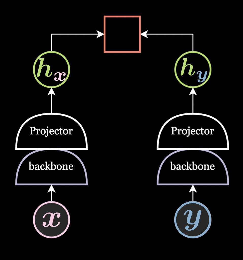Joint Embedding Method, by Alfredo Canziani and Jiachen Zhu

All SSL methods balance two competing forces:

• Invariance: Make representations stable under data augmentations
• Information preservation: Avoid trivial constant outputs (collapse)

Different SSL families handle this trade-off in unique ways.

Core Concepts

Mutual Information (MI)

For two random variables $X$ and $Y$:

$I(X;Y) = H(X) - H(X|Y) = H(Y) - H(Y|X)$

In SSL, we want embeddings $z_1 = f(X)$, $z_2 = f(Y)$ (from two augmented views) that share semantic information (high MI).

The Collapse Problem

If we only minimize $\|z_1 - z_2\|^2$ without constraints, the network collapses to outputting constants, resulting in $I = 0$.

SSL Family Comparison

Different SSL families use different mechanisms to prevent collapse and estimate mutual information:

All modern SSL objectives can be written conceptually as:

$\text{Maximize } I(z_1; z_2) - \alpha R(z)$

where $R(z)$ regularizes representations (avoid trivial solutions).

Contrastive Learning

Core Idea: Learn by discriminating positive (same instance) vs. negative (different instance) pairs.

SimCLR (2020)

SimCLR Illustration, by https://research.google/blog/advancing-self-supervised-and-semi-supervised-learning-with-simclr/

Pipeline:

1. Generate two augmentations of the same image
2. Pass through encoder $f_\theta$ → embeddings $h_1, h_2$
3. Add projection MLP $g_\theta$: $z_1 = g(h_1)$, $z_2 = g(h_2)$
4. Apply InfoNCE loss:

$L_{\text{InfoNCE}} = -\log \frac{\exp(\text{sim}(z_1, z_2)/\tau)}{\sum_{k=1}^{2N} \exp(\text{sim}(z_1, z_k)/\tau)}$

Key Insight: Needs large batches or memory banks for good negatives.

Connection to MI: Oord et al. (2018) proved:

$I(z_1; z_2) \geq \log(N) - L_{\text{InfoNCE}}$

So minimizing InfoNCE maximizes a lower bound on MI.

MoCo (Momentum Contrast)

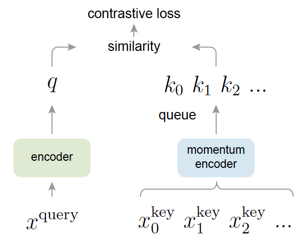MoCo Illustration, by https://doi.org/10.48550/arXiv.1911.05722

Innovation:

• Maintains a momentum encoder and queue of old embeddings as negatives
• Online encoder updates quickly; momentum encoder updates slowly through Exponential Moving Average (EMA)
• Works with smaller batches

Effect: Stabilizes contrastive training without requiring large batches.

Predictive Bootstrap Learning

Core Idea: Predict one view from another without negatives using asymmetry.

BYOL (Bootstrap Your Own Latent, 2020)

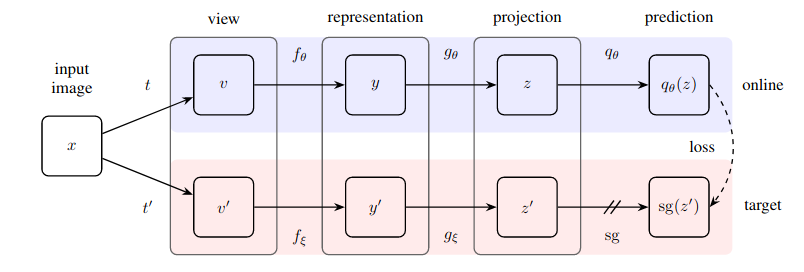BYOL Illustration, by https://doi.org/10.48550/arXiv.2006.07733

Architecture:

• Online network: encoder $f_\theta$, projector $g_\theta$, predictor $q_\theta$
• Target network: encoder $f_\xi$, projector $g_\xi$
• Parameters $\xi$ update via EMA: $\xi \leftarrow m\xi + (1-m)\theta$

Loss:

$L = \|q_\theta(g_\theta(f_\theta(x_1))) - g_\xi(f_\xi(x_2))\|^2$

Why It Works: The slow-moving target stabilizes learning and preserves variance.

SimSiam (2021)

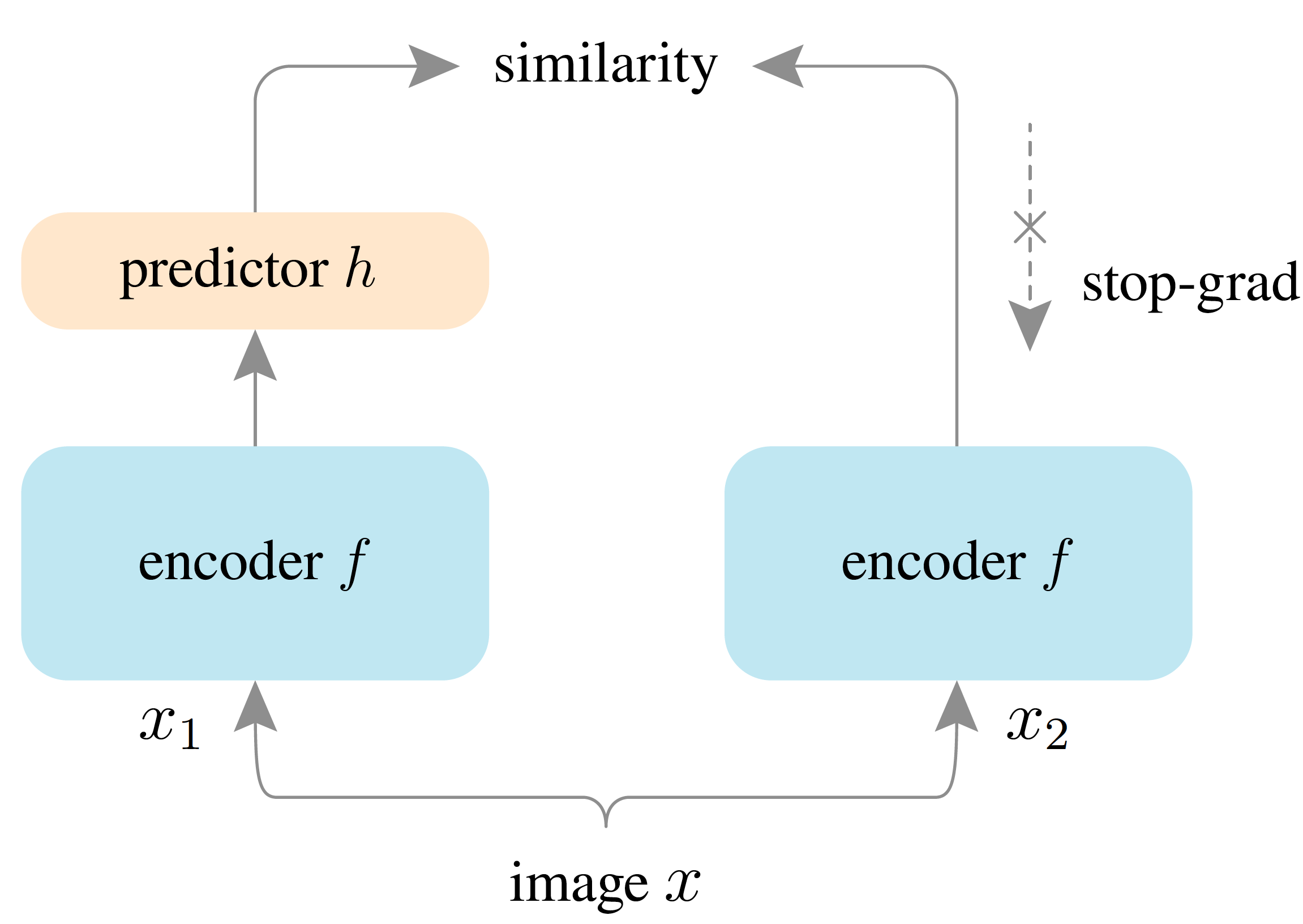SimSiam Illustration, by https://doi.org/10.48550/arXiv.2011.10566

Simplification: No momentum encoder!

Mechanism:

• Two identical branches (same encoder + projector)
• One has a predictor on top
• Crucially: stop-gradient on one branch

Loss:

$L = -\cos(p_1, \text{stopgrad}(z_2)) - \cos(p_2, \text{stopgrad}(z_1))$

Key Insight: Stop-gradient breaks symmetry and prevents collapse by creating asymmetric gradient flow.

DINO (2021)

DINO Illustration, by https://doi.org/10.48550/arXiv.2104.14294

Extension: Scales BYOL-style training to Vision Transformers.

Mechanism:

• Teacher-student setup with EMA teacher
• Both output soft probability distributions (after softmax)
• Loss: cross-entropy between student and teacher outputs
• Uses centering and sharpening on teacher outputs

Emergence: DINO's embeddings show emergent segmentation—ViTs attend to semantic regions without labels!

iBOT (2022)

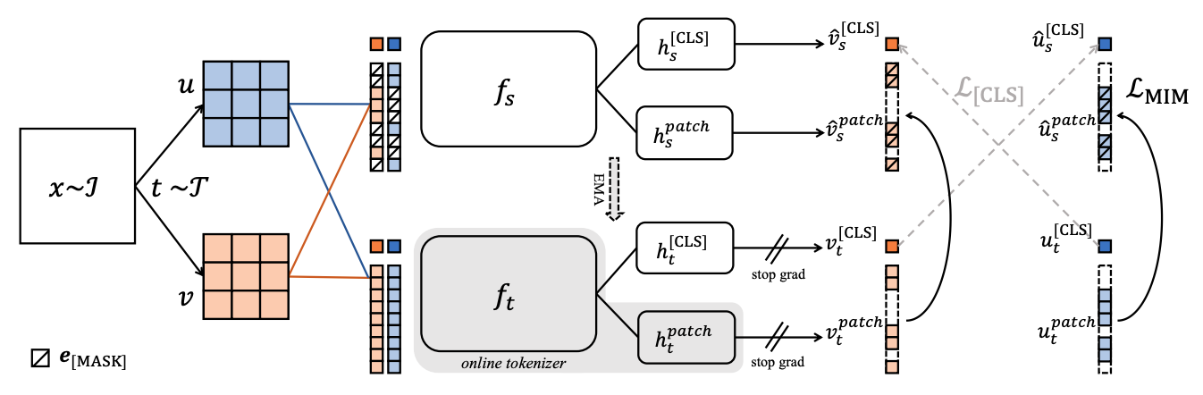iBOT Illustration, by https://doi.org/10.48550/arXiv.2111.07832

Hybrid: Combines DINO + masked prediction.

Innovation:

• Mask random patches of ViT input
• Predict their teacher-assigned tokens
• Unifies predictive and generative principles

Redundancy Reduction

Core Idea: Encourage invariant, diverse, and decorrelated representations.

Barlow Twins (2021)

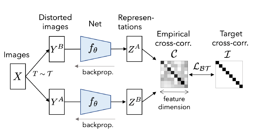Barlow Twins Illustration, by https://doi.org/10.48550/arXiv.2103.03230

Mechanism:

Compute cross-correlation matrix $C_{ij} = \frac{1}{N}\sum_n \frac{z_{1,i}^{(n)} z_{2,j}^{(n)}}{\sigma(z_{1,i})\sigma(z_{2,j})}$

Loss:

$L_{BT} = \sum_i (1 - C_{ii})^2 + \lambda \sum_{i \neq j} C_{ij}^2$

• Diagonal terms → 1: High per-dimension agreement (↑ MI)
• Off-diagonal → 0: Decorrelate features (prevent collapse)

Interpretation: Under Gaussianity, this approximates maximizing per-dimension MI while preventing "all-info-in-one-dim" collapse.

VICReg (2022)

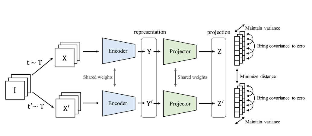VICReg Twins Illustration, by https://doi.org/10.48550/arXiv.2105.04906

Explicit Decomposition:

$L = \lambda_{\text{inv}} \|z_1 - z_2\|^2 + \lambda_{\text{var}} L_{\text{var}} + \lambda_{\text{cov}} L_{\text{cov}}$

Three Terms:

1. Invariance: $L_{\text{inv}} = \|z_1 - z_2\|^2$ (alignment)
2. Variance: $L_{\text{var}} = \frac{1}{d}\sum_j \max(0, \gamma - \text{Std}(z_{\cdot j}))$ (keeps $H(z)$ high)
3. Covariance: $L_{\text{cov}} = \frac{1}{d}\sum_{i \neq j} \text{Cov}(z)_{ij}^2$ (redundancy reduction)

Advantage: Easier to reason about mathematically; no momentum, stop-grad, or large batches needed.

Clustering-based SSL

Core Idea: Group similar embeddings into prototypes and enforce consistent cluster assignments.

SwAV (2020)

SwAV Illustration, by https://doi.org/10.48550/arXiv.2006.09882

Hybrid Approach: Merges contrastive and clustering learning.

Mechanism:

1. Maintain learnable prototype vectors $C = \{c_1, \ldots, c_K\}$
2. For each augmented view $x^{(a)}$, encode to feature $z^{(a)}$ using shared encoder
3. Compute soft assignments $q^{(a)}$ of features to prototypes using Sinkhorn-Knopp algorithm (enforces balanced cluster usage across batch)
4. Predict one view's prototype assignments from another—swap assignments between augmentations

Loss: Cross-entropy between predicted prototype distribution of one view and balanced assignment of the other:

$L = -\sum_i q_i^{(1)} \log p_i^{(2)} - \sum_i q_i^{(2)} \log p_i^{(1)}$

Benefits:

• No explicit negative pairs needed
• Encourages semantic grouping through prototype consistency
• Balanced clustering stabilizes training and accelerates convergence
• Works well even with small batch sizes

Generative SSL

Core Idea: Learn by reconstructing input (or missing parts).

Masked Autoencoder (MAE, 2021)

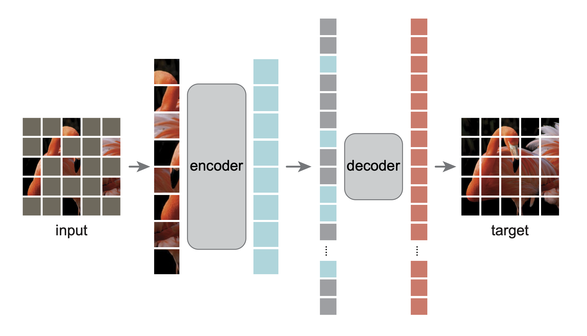MAE Twins Illustration, by https://doi.org/10.48550/arXiv.2111.06377

Mechanism:

• Mask 75% of ViT patches
• Encoder sees only unmasked patches
• Lightweight decoder reconstructs masked pixels
• Loss: MSE on masked patches

Why Effective: Forces encoder to learn global structure without contrastive signals.

Connection to MI: If the decoder models $p_\theta(x_m | x_v)$,

$\mathbb{E}[-\log p_\theta(x_m | x_v)] \approx H(x_m | x_v)$

Minimizing reconstruction ≈ minimizing $H(x_m | x_v)$, thus maximizing $I(x_v; x_m) = H(x_m) - H(x_m | x_v)$.

Mathematical Foundations

Unified Framework

All SSL methods can be viewed as:

$\max_f \underbrace{I(z_1; z_2)}_{\text{alignment}} - \alpha \underbrace{R_{\text{entropy}}(z)}_{\text{avoid collapse}} - \beta \underbrace{R_{\text{redundancy}}(z)}_{\text{spread info}}$

Loss-to-MI Connections

InfoNCE → MI Lower Bound

With similarity score $s(z_1, z_2) = \frac{1}{\tau}\cos(z_1, z_2)$:

$I(z_1; z_2) \geq \log N - L_{\text{InfoNCE}}$

The numerator estimates joint $p(z_1, z_2)$; negatives approximate marginals $p(z_1)p(z_2)$.

Cosine/MSE → MI (Gaussian Assumption)

For whitened, approximately Gaussian representations:

$\cos(z_1, z_2) = 1 - \frac{1}{2}\|z_1 - z_2\|^2 \text{ (first-order on unit sphere)}$

If $(z_1, z_2)$ are jointly Gaussian with correlation $\Sigma$:

$I(z_1; z_2) = -\frac{1}{2}\log\det(I - \Sigma_{12}\Sigma_{21})$

Increasing correlation (reducing $\|z_1 - z_2\|$) monotonically increases MI.

Reconstruction → Conditional Entropy

$\mathbb{E}[-\log p_\theta(x_m | x_v)] \approx H(x_m | x_v)$

Since $I(x_v; x_m) = H(x_m) - H(x_m | x_v)$, reconstruction maximizes MI.

Barlow Twins → Decorrelated MI

Pushing $C_{ii} \to 1$ (high per-dimension MI) and $C_{ij} \to 0$ (decorrelation) prevents redundancy while maximizing information.

VICReg → Explicit Regularization

• Invariance raises $I(z_1; z_2)$
• Variance prevents degenerate low-entropy $z$
• Covariance spreads information across dimensions

Under Gaussianity, these terms are direct surrogates for "maximize MI while preventing collapse and redundancy."

Collapse Prevention Mechanisms

Summary

Key Insights

1. All methods maximize MI between augmented views while preventing collapse
2. Negatives are not necessary — asymmetry (EMA/stop-grad) or explicit regularization suffices
3. Mathematical elegance varies: VICReg is most interpretable, InfoNCE has strongest theoretical foundation
4. Emergence in ViTs: DINO/MAE show that SSL enables semantic understanding without labels
5. Hybrid approaches (iBOT, MSN) combine strengths of multiple paradigms

References

1. Chen et al. (2020). "A Simple Framework for Contrastive Learning of Visual Representations" (SimCLR)
2. Grill et al. (2020). "Bootstrap Your Own Latent" (BYOL)
3. Chen & He (2021). "Exploring Simple Siamese Representation Learning" (SimSiam)
4. Zbontar et al. (2021). "Barlow Twins: Self-Supervised Learning via Redundancy Reduction"
5. Bardes et al. (2022). "VICReg: Variance-Invariance-Covariance Regularization"
6. Caron et al. (2021). "Emerging Properties in Self-Supervised Vision Transformers" (DINO)
7. He et al. (2021). "Masked Autoencoders Are Scalable Vision Learners" (MAE)
8. Zhou et al. (2022). "iBOT: Image BERT Pre-Training with Online Tokenizer"

Conclusion

Self-supervised learning has matured from requiring large batches of negatives (SimCLR) to elegant formulations based on redundancy reduction (VICReg) and masked prediction (DINO). The key insight is that meaningful representations emerge when models balance invariance to augmentations with preservation of information diversity.

The field continues to evolve, with recent work focusing on:

• Scaling to billion-image datasets (DINOv2, SEER)
• Multi-modal learning (CLIP, Data2Vec)
• Efficient training (faster convergence, lower compute)
• Theoretical understanding (why does stop-gradient work?)

Understanding these fundamentals provides a strong foundation for both using and extending self-supervised learning methods.