Image to video, from first principles: a six-lesson course
A six-lesson, hands-on course on image-to-video generation that you can follow step by step. Start with why a pixel-MSE predictor averages uncertain futures, then add diffusion, flow matching, temporal attention (and a JEPA detour), generate real robot video in a learned latent space, and finish by adapting a pretrained LTX-Video 2B with LoRA. Every lesson changes one factor, keeps its controls, and shows its failures. Lessons 1–5 train every weight from scratch.
Most explanations of video generation start with a finished system: a huge Transformer, a video VAE, a billion frames. It is hard to tell which part does what. This course goes the other way. It starts with a 4×4 white square on a 32×32 black canvas, builds one mechanism per lesson, and ends with a pretrained 2-billion-parameter generator that I adapt myself.
The through-line is one sentence:
Predict one future → represent many futures → learn a sampling path → let frames communicate → compress real video → train and evaluate a useful system.
- Lessons
- 6 notebooks
- Trained from scratch
- Lessons 1–5
- Toy task
- 32×32 square, 7 future frames
- Capstone
- LTX-Video 2B + LoRA
How to use this post
Read the lessons in order; each one builds on the last. Every lesson has the same five beats:
- The question it answers.
- The setup: data, model, and what is held fixed.
- Walk-through: figures and looping clips, each with a Watch for note that tells you what to look at before you press play.
- The result, with the numbers.
- Carry forward: what to keep, and a question to check yourself.
Four rules hold throughout:
- One factor at a time. Objective, architecture, representation, conditioning and training scale are separate choices. Flow matching does not need a Transformer. A Transformer does not guarantee coherent motion. JEPA predicts representations, not pixels.
- Controls and failures stay in. Later lessons are not guaranteed to beat earlier ones, and several don't.
- Honest splits. In the toy lessons, starting positions are split before clips are generated (140 train / 40 validation / 45 test positions). In Lesson 5, whole trajectories are held out. In Lesson 6, clips are grouped by source video.
- Diagnostics, not leaderboards. Pixel MSE against one recorded future is a diagnostic, not a quality score: a different but plausible future can score badly, and a frozen frame can score deceptively well.
| Lesson | The question | What it shows |
|---|---|---|
| 1 · Deterministic prediction | Why does a CNN average conflicting futures? | Prediction vs. the exact conditional mean |
| 2 · Diffusion | How can one image give different coherent futures? | Sampled futures, denoising, coverage |
| 3 · Flow matching | What changes with a velocity field? | Integration, solver steps, matched comparison |
| 4 · Temporal attention | How do future frames agree on a trajectory? | Ablation, scaling failure, JEPA |
| 5 · Real video from scratch | Can learned compression handle RGB video? | Reconstruction ceiling, robot futures, failures |
| 6 · Practical capstone | Can a small run improve a pretrained generator? | Paired base vs. adapter videos |
Lesson 1 · Why a predicted video becomes an average
The question. When does one image determine a future, and when must a predictor average alternatives?
1.1 Setup: a world small enough to understand
Every clip has a 4×4 square in eight 32×32 grayscale frames. The input is frame 0, and the other seven frames are the targets. The image tells you where the square starts. The dataset supplies the motion rule. In the right-only dataset the rule is always one pixel right per frame, so the future is determined even though one frame shows no velocity.
Starting positions are split before any clip is generated, so validation and test positions never appear in training.
Watch for. The only thing the image carries is the start position. Nothing in a single frame says which way the square will move.
1.2 The model: one CNN, seven output channels
A four-layer CNN reads the image and outputs seven channels, one per future frame. All channels share the same learned features and are trained together against a whole target clip. There is no recurrence and no attention. The network learns a fixed short-horizon mapping, trained with pixel MSE: compare every predicted pixel with its target, backpropagate, update. Each run is 40 epochs and keeps the checkpoint with the lowest validation MSE.
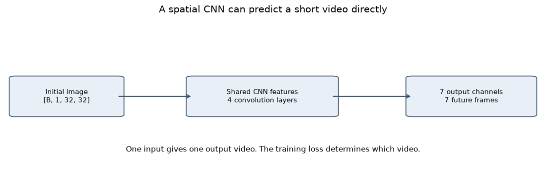
1.3 When the future is determined, the CNN is fine
Watch for. Both panels show a crisp square moving right. This is the baseline: when the answer is unique, MSE regression works.
1.4 Now make the future ambiguous
Keep each input image identical but pair it with every allowed direction, equally often: two, four or eight. The model receives the image and no direction label. It must return one video for all of those conflicting targets.
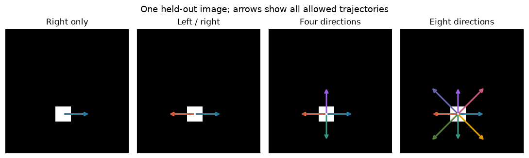
With MSE, the best deterministic answer is the conditional mean:
For two non-overlapping futures, committing to one trajectory gets the other wrong. Predicting half brightness at both locations splits the error and lowers MSE. With four or eight alternatives, each square fades toward ¼ or ⅛ brightness, and overlaps add up. An accurate average can be an invalid video.
1.5 Watch the average appear
Each clip below plays all the valid futures beside the exact mean and the CNN's output.
Watch for. (1) The CNN panel is nearly identical to the exact-mean panel, so the network did learn well. (2) The more directions there are, the fainter and more smeared the mean. No panel of the mean looks like a real video.
1.6 Separate ambiguity from incomplete learning
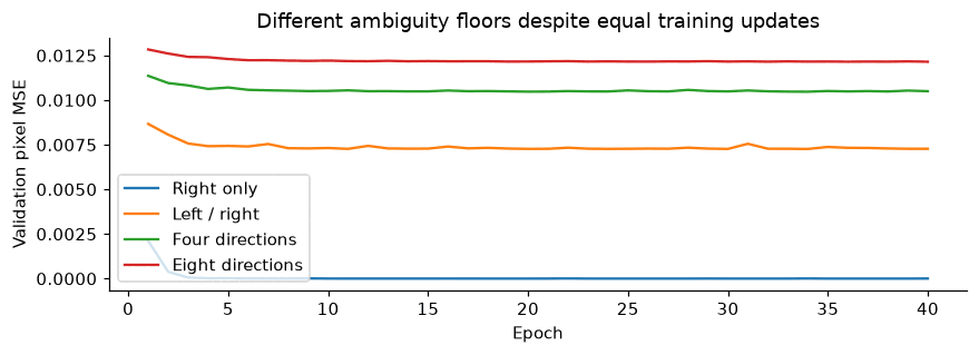
Two different things can make the loss high, and they must not be confused:
The generator is known, so the exact mean is an analytical benchmark. A CNN that plateaus right at the benchmark has learned the ambiguous task perfectly. It is the task that forbids a sharp answer.
1.7 The control: give the model the missing information
Concatenate two constant maps, dx and dy, to the image. Now the input says
which trajectory to predict, the conditional mean becomes that one trajectory,
and the optimal MSE is zero.
Making the network bigger would not have fixed Figure 1.5. The missing ingredient was information, not capacity.
Carry forward. If you want several futures from one image, you need a distribution and samples, not a better regressor.
Check yourself. Why can a faded two-square average have lower MSE than a sharp, valid trajectory?
Lesson 2 · From an average to sampled futures
The question. How can the same image produce several sharp, coherent futures?
2.1 Setup: learn a distribution, then draw from it
Instead of one video , learn and draw a video from it. The data is exactly Lesson 1's: 140 / 40 / 45 positions, which gives 280 / 80 / 90 clips for balanced left/right motion. Future pixels are normalized to .
2.2 Add noise to a known future
Training starts from a real clip, moving left or right. Pick a noise level uniformly from 0 to 99, draw independent Gaussian noise for every future pixel and frame, and mix:
Here falls from about 1 (clean) to about 0 (pure noise) as goes from 0 to 99, so is how much signal remains and how much noise. The clean first frame is kept as a condition. One noise level applies to the whole clip, and diffusion level is separate from video-frame time. Left and right use the same noise distribution, so noise carries no direction label.
2.3 Learn to denoise, then generate
The denoiser sees noisy future + noise level + clean first frame and predicts the noise that was added. At generation time there is no target: start from fresh Gaussian noise and apply 100 reverse steps to all seven frames together.
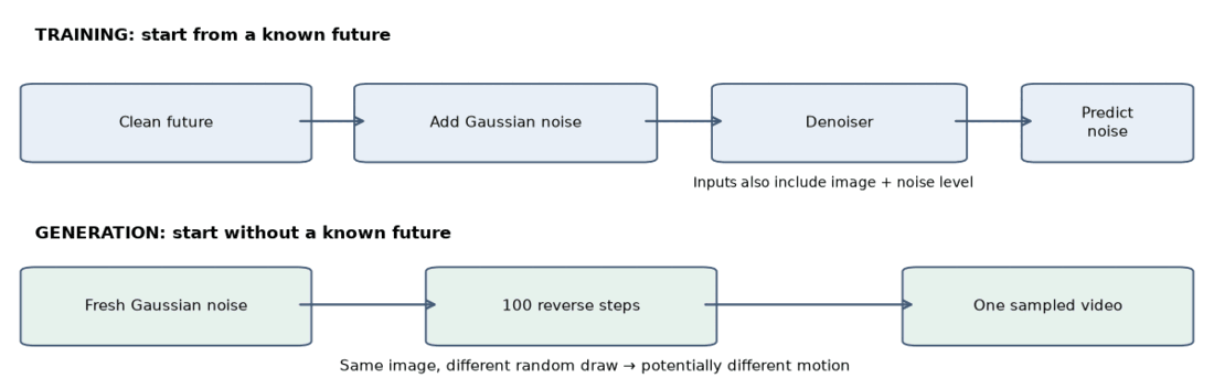
There is no left/right decision head. Why doesn't this average again? Because the denoiser sees the noisy clip, not just the image. A noisy state that already leans toward the right-moving future is cleaned toward the right; one that leans left is cleaned toward the left. The averaging that remains is only among futures consistent with that state, not among all futures of the image.
2.4 Make the sampler work: three controlled experiments
A valid objective does not guarantee a working sampler. Same data, 60 epochs, 100 reverse steps, left/right only:
| Experiment | What changes | Intuition |
|---|---|---|
| Small 3D CNN, epsilon target | Starting model | Mix nearby frames and pixels |
| Video U-Net, epsilon target | Architecture | Broad spatial context, skip connections, explicit frame positions |
| Video U-Net, v target | Training target | Avoid dividing by a near-zero signal scale |
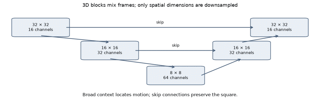
Why the target matters. For , epsilon prediction reconstructs , and when is tiny a small noise error becomes a large video error. The alternative gives with no division. Diffusion's is not the square's velocity and not flow matching's field.
Scoring uses a rule stated up front. The nearest-trajectory MSE of a clip is its MSE to the closest exact clip among the valid directions. A clip is plausible if that MSE is below 0.005, the closest direction is the same in every frame, and the foreground is 12–20 pixels in every frame (the square has 16, with some tolerance). This is a toy heuristic, not a general video metric. Evaluation is 8 held-out images × 8 draws = 64 clips.
| Model (left/right) | Plausible clips of 64 |
|---|---|
| Small 3D CNN, epsilon | 0 |
| Video U-Net, epsilon | 41 |
| Video U-Net, v target | 64 |
Watch for. Panels 1–2 are the smeared average. Panels 3, 4 and 5 are the small diffusion CNN (0/64 plausible), U-Net epsilon (41/64) and U-Net v (64/64). Look for squares that flicker, change size or switch direction in the weaker models.
2.5 Eight unfiltered draws
Watch for. Each draw commits to one trajectory, and different draws choose different directions. Nothing is blended.
2.6 Watch one draw develop a direction
Each clip pairs the noisy state (left) with the model's current clean estimate (right), across the 100 reverse steps. Both draws start from the same image. "Right" and "Left" only label how each draw ends; they are not inputs.
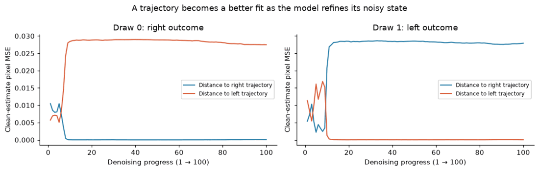
Watch for. Early on, the clean estimate is a faint smear of both alternatives. Within roughly the first ten of 100 steps it separates toward one side and stays there, although the noisy state remains noisy for much longer. In Figure 2.7 the curves cross and then diverge sharply. This is an observation from these draws, not a fixed selection stage: there is no direction head and no irreversible lock-in.
2.7 Where do the possible directions come from?
From the training examples, not from the noise. For every starting image, the data generator creates one clip per allowed direction. The direction is used to make targets; it is never given to the denoiser.
| Dataset | Valid directions per input | Train clips | Intended probability each |
|---|---|---|---|
| Right only | 1 | 140 | 1 |
| Left/right | 2 | 280 | ½ |
| Four directions | 4 | 560 | ¼ |
| Eight directions | 8 | 1,120 | ⅛ |
2.8 Audit: check the failures before trusting the counts
A sharp-looking frame need not be part of a valid trajectory. I flag three overlapping problems: the nearest direction changes across frames, the foreground size leaves 12–20 px, or the trajectory MSE exceeds 0.005.
Over 45 test positions × 32 draws = 1,440 clips per dataset, using fresh seeds, the counts of plausible clips are:
| Dataset | Plausible of 1,440 |
|---|---|
| Left/right | 1,440 |
| Four directions | 1,438 |
| Eight directions | 1,390 |
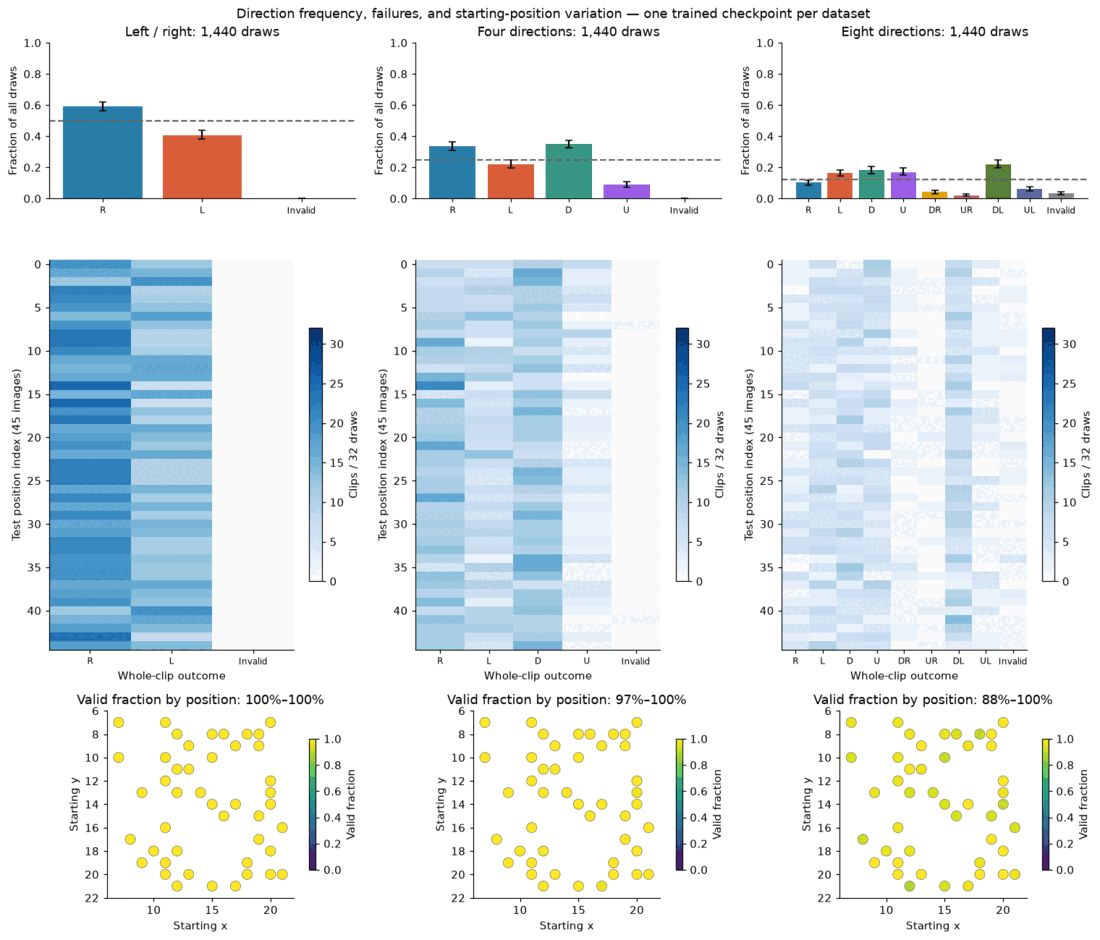
Carry forward. Sampling removes the averaging, and nearly every clip is valid. But a valid clip does not mean a correct probability: Figure 2.10 also shows how often each direction is chosen, and whether that matches the intended share is the question the next lessons keep asking.
Check yourself. Why does independent Gaussian noise, with no left/right label, still let generated videos move in either direction?
Lesson 3 · Flow matching: learn a path to video
The question. What changes when we predict a velocity field instead of a denoising target?
3.1 Setup: same task, same U-Net, new path
Keep the data, the conditioning and the U-Net layers. Change the path and the sampler. The training budget is 60 epochs × 1,120 examples, batch 16, Adam at 0.001, with checkpoints chosen on fixed validation noise and times.
Three time symbols appear in this post, so here they are once:
| Symbol | Where | Meaning |
|---|---|---|
| Lesson 2 | Diffusion step, 0–99. High means noisier | |
| Lessons 3–5 | Flow time, 0 to 1. 0 is noise, 1 is data | |
| Lesson 6 | Noise level, . 1 is noise |
None of these is video-frame time, which is always the seven (or 49) frames.
3.2 Construct a path from noise to a known future
Take a target video and independent Gaussian noise , and define
At the state is noise, and at it is the target. The clean first image is kept as the condition. This is a constructed training path, not a model prediction. And is generation time, separate from the seven video-frame times.
Watch for. As τ increases, the noise fades and the square emerges. Nothing here is learned yet; it is just the interpolation we will train against.
3.3 Predict the velocity along that path
Differentiate the interpolation:
This velocity is a video-shaped tensor describing how pixel values change along generation time. It is not the square's and it is not diffusion's . Train with velocity MSE. For each example draw fresh noise and a uniform . No ODE solve is needed in training.
The network learns the average target velocity conditioned on the current state, time and image. That defines a field that transports a distribution of states. It does not return one averaged finished video from the image alone. Why this avoids Lesson 1's problem: the input now includes the noisy state . Different noise draws sit in different places, so the best velocity at each state points toward one specific future. Averaging happens only among futures consistent with that state.
3.4 Follow the field to generate
Start from fresh noise and integrate . This is an ODE: a deterministic rule for how the state changes. An Euler step simply moves the state a small straight step along the current velocity: . Each step updates all seven frames together. No noise is injected after initialization, so with the same model, noise and solver the path is deterministic. Different initial noise can end in different motion modes.
As a sanity check on the equations and solver I first integrated an oracle field that knows the target; it reproduced the target to about 10⁻⁶ at 1, 10 and 100 steps. That verifies the implementation, not learned quality.
Watch for. As in Lesson 2, each draw commits to one trajectory. Count how many go each way.
3.5 Watch a direction develop during integration
The clean estimate at any time is
For the known straight training path this identity is exact. For a learned field it is a diagnostic estimate, not the result of integrating the rest of the path.
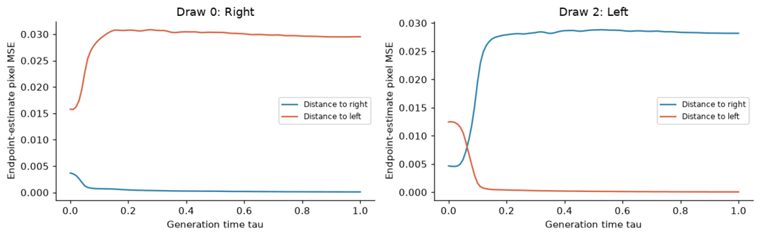
Watch for. Near τ = 0 the estimate is a faint blend of alternatives; the two distance curves in Figure 3.5 separate early (by about τ = 0.1–0.2), then the chosen direction sharpens.
3.6 Diffusion and flow side by side
Both start from the same Gaussian tensor. DDPM adds fresh noise between updates, while the flow ODE follows its learned field. Equal update counts do not mean equal noise strength.
Watch for. Both start from identical noise. DDPM re-injects noise between updates, so its state stays grainy until late. The flow state is a deterministic path and sharpens steadily.
3.7 How many field evaluations are enough?
A straight training path does not imply one learned Euler step is enough, since a single step cannot adapt to the changing state. On a separate validation subset (8 images × 8 draws, identical initial noise):
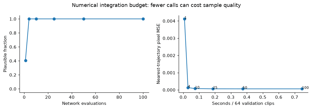
One step gives only 26/64 plausible clips, but four steps already give 64/64, and more steps shave pixel error slightly. This concerns left/right motion on a small validation subset; it does not establish a general speed advantage over diffusion.
3.8 Is flow better than diffusion here? Not on motion quality
Same image, same U-Net, same budget, consecutive draws from both samplers:
On eight directions (64 clips here), diffusion produced 62 valid clips against 44 for flow. Among valid clips the acceleration, which is how much the frame-to-frame speed changes (lower is smoother), was 0.021 vs. 0.057 px/frame². A smooth generation path is not the same as smooth video motion. There is no evidence here that flow makes motion smoother. Its benefit in this experiment is the simple velocity objective and a usable low-step sampler.
3.9 Audit: sharp is not calibrated
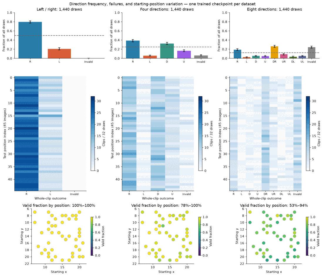
- Left/right: valid in 1,440/1,440 draws, yet 1,144 (79%) move right instead of the intended 50%.
- Four directions: 1,347/1,440 valid (94%).
- Eight directions: 1,090/1,440 valid (76%), with 242 direction-change flags. Per-position success ranges from 53% to 94%.
Crisp motion does not guarantee correct probabilities or uniform reliability. These are single runs with finite draws.
Lesson 3 recap
| Method | What it learns | How it generates |
|---|---|---|
| Direct CNN | A finished video from the image | One deterministic output; MSE averages ambiguity |
| Diffusion | Denoising quantities at noisy states | Iteratively samples a video distribution |
| Flow matching | Velocities along noise-to-video paths | Integrates a field from a random starting state |
3.10 Optional extension: beyond the trained horizon
The U-Net accepts a variable temporal length but only learned seven frames. Asking for 20 stretches its frame-position coordinate. It is not a trained prediction of times 8–20. I compared two strategies on one held-out start whose square stays on the canvas: generate 20 frames jointly, or generate seven, feed the last frame back, and repeat.
Watch for. After frame 7 (beyond what was trained), see which version keeps the square moving at the right speed.
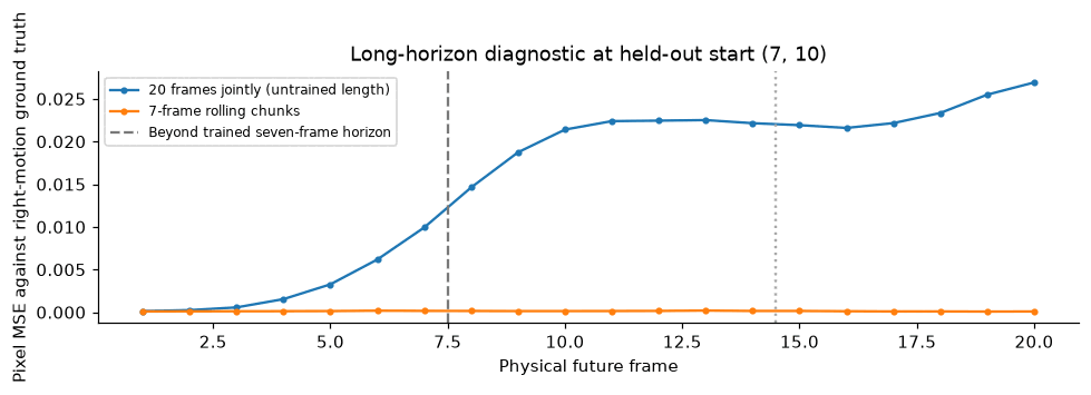
The joint request gives slow, blurred motion (frames 8–20 MSE 0.0220) and rolling tracks the target (0.00013). It also changes both the temporal coordinate and the input length, so the cause isn't isolated. One right-moving case shows a mechanism, not robust long-horizon performance.
Carry forward. Both generative methods can represent alternatives. Neither guarantees realistic samples, correct direction frequencies or efficient sampling. Judge those separately.
Check yourself. Why can velocity MSE support multiple futures while direct video MSE averages them? Why does a deterministic ODE still produce diverse videos?
Lesson 4 · How future frames communicate
The question. What does temporal attention contribute to a coherent video?
4.1 Setup: why leave the U-Net?
Lesson 3's U-Net gives valid left/right motion but biased frequencies, and only 1,090/1,440 eight-direction clips pass the toy checks, with per-position success ranging from 53% to 94%. Those are limits of this model and recipe, not proof that U-Nets cannot generate realistic video. Convolutions bring shared local filters; attention brings adaptive long-range connections but needs more optimization and data. Here is one concrete failure:
4.2 Turn the future video into tokens
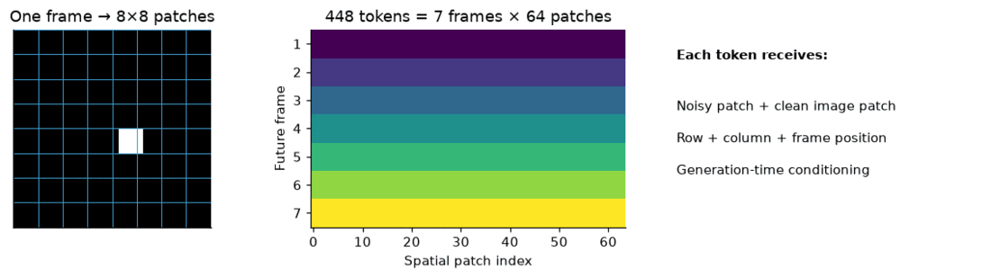
The token recipe:
- Split each 32×32 frame into 64 patches of 4×4 pixels. Seven frames give 448 tokens of 128 features each.
- Linear layers embed the noisy pixels and the matching clean-image patch.
- A small framewise convolutional stem adds local features. It never mixes future frames.
- Learned row, column and frame embeddings say where each token belongs, and generation time has its own embedding.
- The output layer predicts 16 pixel velocities per token.
Patchifying rearranges pixels; it does not compress anything.
4.3 Alternate spatial and temporal attention
Attention computes : each token becomes a weighted mix of others' features. Spatial attention lets a frame's 64 patches talk to each other. Temporal attention lets the seven tokens at one patch location talk across frames. Alternating them moves information between places and times. I use three blocks with four heads. Both directions are bidirectional, because the whole future is generated jointly.
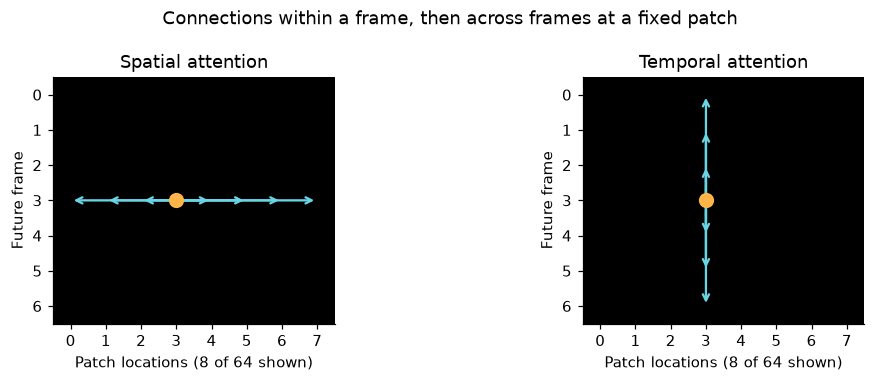
The model has 763,088 parameters. The objective is Lesson 3's: the same linear path and velocity target. Only the architecture changes.
4.4 Train on the same uncertain futures
Train from scratch for 60 epochs × 1,120 examples, then continue the selected checkpoint for 120 more epochs with the optimizer state restarted (180 total). The U-Net baseline stays at 60 epochs, so improvement after continuation cannot be credited to architecture alone.
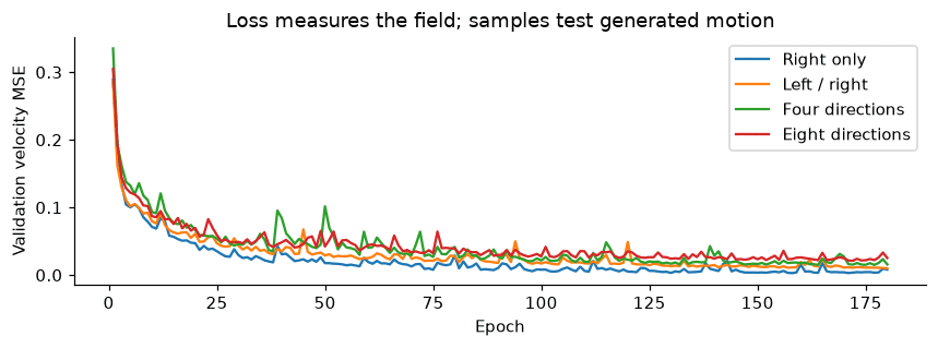
The Transformer did not win. A plain patch Transformer produced 0/64 valid left/right clips at 60 epochs (that run is archived). With the convolutional stem and longer training it improved, but at 60 epochs the U-Net still won in every direction set, and on eight directions the Transformer reached only 1/64 valid clips.
4.5 Look at whole clips, including failures
Watch for. Compare the two clips. Left/right draws are mostly valid (72% overall in the audit below), while eight-direction draws mostly fail the checks (1% valid), so look for squares that change size or direction between frames.
4.6 The key experiment: remove communication between frames
Keep spatial attention, image conditioning, frame positions and flow matching. Skip every temporal-attention layer. Each frame now starts from its own independent noise, and a frame can look right while its neighbors pick a different direction. Both versions use the same 60 + 120 epoch protocol. The no-attention model has fewer active parameters, so the comparison is not equal compute.
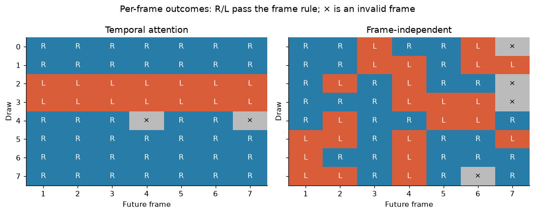
| Model | Frames passing the checks | Whole clips valid |
|---|---|---|
| With temporal attention | 403/448 | 57/64 |
| Without | 379/448 | 2/64 |
(Left/right, 8 images × 8 draws = 64 clips here; the 1,440-draw audit in 4.8 uses a larger sample, so its percentages differ.) Individual frames look fine either way. Without communication they simply disagree. Even with perfect frames, seven independent 50/50 choices give only probability of one consistent direction. Temporal communication is what coordinates the choice.
4.7 Inspect the learned temporal connections
At generation time 0.5, for one spatial patch in the last block, rows are the querying frames, columns the frames supplying features, averaged over four heads, and each row sums to one.
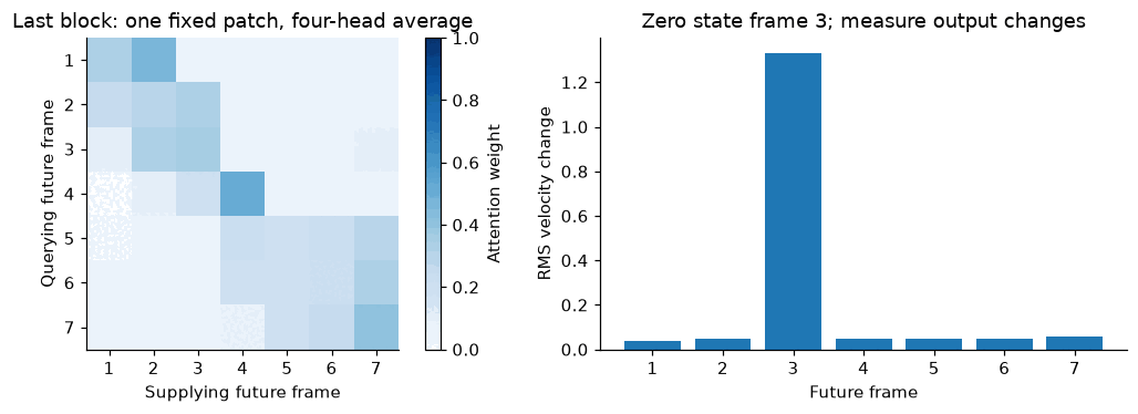
Read this carefully. The attention map is a diagnostic, not a motion probability. In the influence test on the right, zeroing frame 3 changes frame 3's own output by far the most (RMS about 1.3, against roughly 0.05 for the other frames). So this single test shows only weak dependence between frames, and no hard rule forces the same direction across frames. It does not show how attention coordinates direction. The ablation in 4.6 is the real evidence.
4.8 The scaling audit
Over 45 positions × 32 draws, using the 180-epoch Transformer:
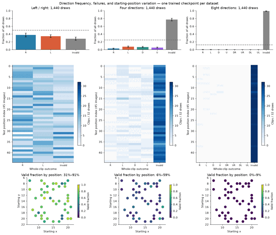
- Left/right: 1,039/1,440 valid (72%), with per-position success from 31% to 91%.
- Four directions: 327/1,440 (23%).
- Eight directions: 15/1,440 (1%).
The small illustrative batch looked far better than this, which is the case for the larger audit. For scale, the 60-epoch U-Net passes 1,090/1,440 eight-direction clips (Lesson 3) against the Transformer's 15.
4.9 Detour: JEPA, which predicts features rather than pixels
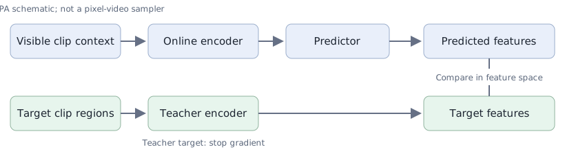
The question: can we predict the future in feature space instead of pixel space, and does that remove the averaging problem? An online encoder reads the observed frame(s), a predictor forecasts seven future embeddings, and a teacher encodes the real future only to build targets. The teacher is an exponential moving average (EMA), meaning a slow running average of the online encoder's weights, and "sg" means stop-gradient: treat that term as a constant.
Here supplies one image and supplies two observed frames, mixed randomly in training. A separate pixel probe decodes features so we can see them.
| Context | Nearest-direction accuracy (how often the forecast is closest to the recorded direction) | Decoded pixel MSE |
|---|---|---|
| One image | 12.5% (chance for 8 directions) | 0.0156 |
| Two frames | 99.7% | 0.0031 |
The whole run took about 6.5 seconds. One image holds no direction evidence, so a deterministic feature predictor cannot pick the recorded alternative. Two frames expose the motion. The teacher probe's own reconstruction error (0.0002) separates a poor forecast from a poor decoder. JEPA gives a predictive representation for understanding and planning, but it still needs another mechanism to sample sharp pixel futures. That job belongs to diffusion and flow matching.
Carry forward. Attention shares information; it is not an automatic upgrade. It matters when frames must agree, and it is data-hungry. JEPA answered its question only in part: feature prediction works once the motion is observable, but it does not sample pixel futures.
Check yourself. If every frame is individually perfect, why can the whole clip still be wrong?
Lesson 5 · Real video: compression and uncertain motion
The question. Can learned compression support generation of real RGB futures?
5.1 Setup: the task, the data and an honest split
The BAIR robot pushing set has real 64×64 RGB robot videos. Three official training shards give 768 trajectories, a fourth shard gives 256 for validation, and the separate official test shard gives 256. No test trajectory enters training. Two 11-frame windows per trajectory (starting at source frames 0 and 15) stay together.
The model predicts frames 4–10 in both settings:
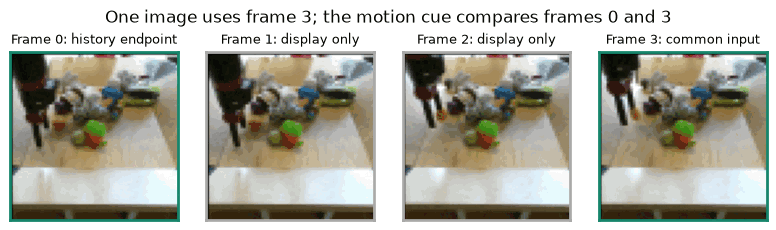
- One-image: sees only frame 3.
- History cue: frames 0 and 3. This is a coarse endpoint cue, not the full history. It is supplied as , the average per-frame change.
Actions and robot state are ignored.
5.2 Preserve the scene before generating motion
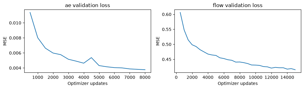
Train a frame autoencoder: 3×64×64 pixels → 8×16×16 latents → RGB pixels. It has 498,571 parameters. Each frame is encoded independently, with no temporal compression and no pretrained perceptual network. Pixel MSE plus a spatial-gradient loss trains it, and validation MSE picks the checkpoint. Compression failure and future-generation failure are different problems, so check reconstruction first.
Watch for. Compare the right panel with the left one for lost detail (arm edges, small objects). This is the ceiling: the generator can never be sharper than its decoder.
5.3 Model future changes in latent space
Freeze the autoencoder, standardize its channels, and model each future as a latent change from the last observed frame:
Train with flow matching on and target velocity . At sampling time, integrate and recover before decoding. The generator (1,329,288 parameters) is a local 3D conv followed by four Transformer blocks that alternate spatial attention over 256 positions with temporal attention over seven futures. The observed latent frame is given at every future position. For the history setting, the coarse cue is added; one-image mode gets a zero cue and an explicit missing-history flag. Here is the training-set standard deviation of latent changes, per channel.
5.4 Sample the next move
Here are the first four official held-out trajectories, first window, not selected for looks. Clips begin at frame 3, the common last observed frame, followed by seven futures. One-image uses two independent seeds. History uses the first seed. Draws A and B use different seeds. The history draw reuses seed A, so any difference from A comes from the extra cue, not from luck of initialization.
Watch for. The frozen column never moves. Check whether the generated columns move, whether the two one-image draws differ from each other, and whether the arm keeps its shape; the audit below reports blur and shape errors.
5.5 Audit: motion, alternatives and failures
I evaluate the first window of all 256 test trajectories, one sample per condition, so overlapping windows aren't counted as independent. The recorded future is one continuation. Plausible alternatives can score poorly.
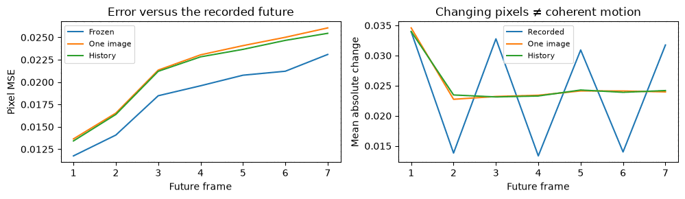
- The history cue lowers recorded-future MSE by about 1.4% (0.02139 → 0.02109). The paired trajectory-bootstrap interval favors history, but the effect is small.
- Generated motion magnitude is close to the recordings (0.0252 vs. 0.0244), and the generated lines are steady where the recorded line zigzags.
- The frozen frame has the lowest MSE at every future frame while producing no motion at all. Mean absolute change near zero means freezing, while too much can mean flicker.
- Diversity is reported separately: 0.051 is the mean pixel difference between the two one-image draws. Sampling takes about 0.06 s per clip.
Watch for. Where does the generated arm or object depart from the recording? A large MSE can come from a plausible alternative, not just from an error.
I show the worst cases instead of hiding them. No claim about FVD (a standard video-quality score) or perceptual quality is made from these diagnostics.
Carry forward. The pieces now fit: RGB clips → learned latents → conditional sampling → decoded clips. Compression and dynamics must both work, and a poor decoder cannot be rescued by a better sampler. The history cue uses only two frames, and unknown robot commands still leave uncertainty.
Check yourself. Why can a frozen frame beat a good generator on pixel MSE, and what should you measure instead?
Lesson 6 · A practical capstone: adapt a pretrained generator
The question. Can a small training run improve a pretrained video generator on a narrow motion task?
Here I stop training from scratch, and say so. LTX-Video 2B brings its general image and video knowledge from pretraining. Any gain from my adaptation has to be shown with held-out evidence.
6.1 Choose a visible, narrow behavior
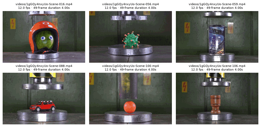
The task is hydraulic-press object deformation from the public crush-smol pilot. The first image supplies the object and scene, the caption supplies the requested action, and the model must keep identity while geometry changes.
- Split: 38 train / 3 validation / 6 test clips, grouped by original-video ID (7 / 2 / 2 source groups). Object independence is unverified, and captions are machine-written.
- Retained frames: 49 uniformly spaced frames covering the complete action, center-cropped to 512×320 and played at 12 fps (about four seconds). This normalizes action duration and changes original speed.
6.2 Put the mechanisms together
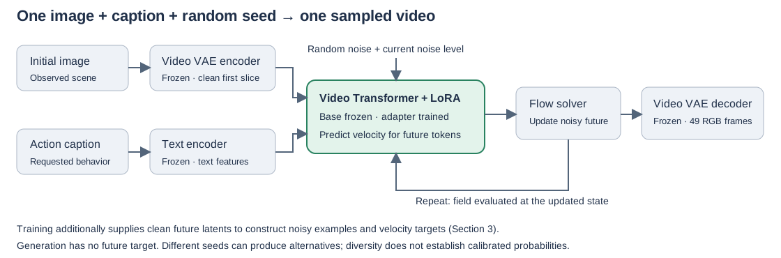
A temporally compressed VAE turns 49 frames into seven latent time slices on a 16×10 grid, so the Transformer processes 7×16×10 = 1,120 tokens. The first slice carries the image condition and the other slices are sampled jointly. The VAE needs spatial sizes divisible by 32 and a frame count of 8k+1; 512×320×49 is a practical bucket, not a duration limit. This is a real change from Lesson 5's independently encoded frames.
The text encoder, video VAE and base Transformer are frozen and pretrained. Only attention-layer LoRA parameters train:
LoRA freezes the weight and learns a low-rank correction (rank , scale ). That is 14.68M of 1.94B Transformer parameters (0.76%).
6.3 The exact training example
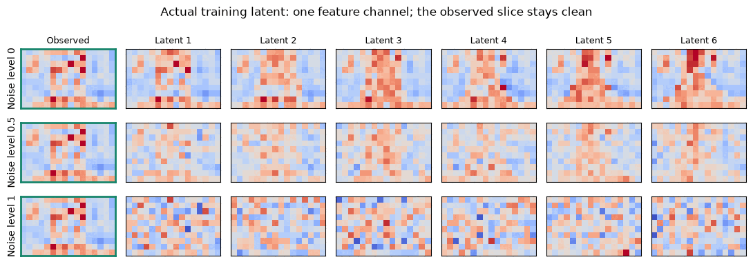
With clean latents , noise and level , future tokens are
First-frame tokens stay clean, get timestep zero and are excluded from the loss, so every example is conditioned on its first frame. This runs in the opposite time direction to Lesson 3: with , , which is the same motion with a sign flip. And this is linear-path flow velocity, not Lesson 2's diffusion- (which comes from the mixing).
6.4 Measure feasibility, then train
A 20-update pilot used 11.4 GiB on an A40 at about 0.7 s per update. It establishes memory feasibility, not quality. The main recipe is 1,500 updates, batch 1, rank 16, and took about 10.5 minutes of training.
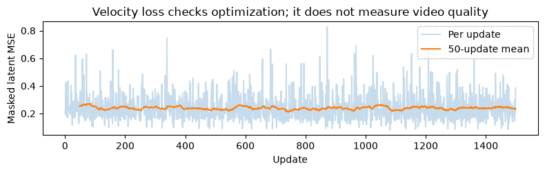
Read this. The loss is flat and noisy. That is why quality is judged on videos, not on this curve.
Checkpoint selection. I compared 500, 1,000 and 1,500 updates on the same three validation images and two seeds, and fixed the choice before any test generation:
| Candidate | Validation observation |
|---|---|
| 500 | Stronger action than base in several draws; the small-candy case often stops near contact |
| 1,000 | More action, but conspicuous press-geometry changes in case 00 |
| 1,500 | Clearest action on the hardest case; still invents debris and transfers appearance |
I chose 1,500 updates, and that adapter is "the adapter" in everything below. The choice favors visible action and does not dominate every fidelity criterion.
6.5 Compare videos before making any quality claim
Base and adapter are run with identical held-out image, caption, seed, fps, frame count, inference steps, guidance and conditioning noise: 6 test cases × 2 seeds = 12 draws per model. Each clip below shows recorded alternative | base | LoRA adapter.
Watch for. In each clip, compare the middle panel to the right one at the moment of contact. Then look at the press itself in Figure 6.8.
| Test case | Base | Adapter |
|---|---|---|
| 00 · thin-tool rig | Preserves the rig, little motion | Replaces the thin tool with a broad cylinder: hardware failure |
| 01 · colored stack | Limited compression | Stronger flattening in both seeds; unstable fragments |
| 02 · green/orange disks | Seed-dependent contact | Better contact in one draw; limited extrusion |
| 03 · pink pile | Mostly approach and contact | Clearer compression; some press and texture drift |
| 04 · sparkly sphere | Partial squash; invents a metal bar | Stronger flattening; the recorded clip crumbles instead |
| 05 · lime | One burst, one weak-motion draw | Both draws crush and spill |
Interpretation. The adapter makes compression more visible on several held-out objects but doesn't reliably preserve machinery or material behavior. Yellow markings appearing on a previously plain shaft suggest appearance transfer from the training scenes. That is a plausible diagnosis, not a causal ablation. This is a useful action demo with identifiable failures, not a physics simulator.
What this does not claim.
- The review is descriptive: frames 0, 12, 24, 36 and 48 of all 12 draws per model, with the full videos retained.
- It is not a blinded human study and gives no success rate.
- Two independent source IDs cannot support a confidence interval.
- Case 04's different breakup alone doesn't prove failure, since its caption asks for flattening.
Carry forward. The adapter learns correlated appearance and motion together. Judging identity and action separately is the next improvement.
Check yourself. Which parts of the result come from LTX's pretraining, and which from my 0.76% of trained parameters?
What I took away
- Averaging is MSE's default under ambiguity. If the task has several valid futures, the fix is a distribution and a sampler, not a bigger network.
- Diffusion and flow matching both represent alternatives. Neither guarantees calibrated probabilities, uniform reliability or smooth motion. Count invalid clips instead of hiding them.
- Check controls before crediting the fancy part. The U-Net beat the small Transformer, the ablation showed what attention is actually for, and the frozen frame beat the generator on MSE.
- Small illustrative batches mislead. Several conclusions changed between a batch of eight and 1,440 draws.
- Separate what is pretrained from what you trained. In the capstone the general visual knowledge is LTX's. Only the narrow, measurable change is mine, and its failures are as informative as its wins.
Where this goes next
- A 75% / 25% left/right training mix: does the sampler reproduce the intended probabilities?
- A larger capstone audit: 12 source-disjoint cases × 4 seeds × 2 models, assessing identity, action, temporal consistency and severe failures separately, with a blinded preference check and bootstrap over cases.
- A temporally aware video autoencoder in place of Lesson 5's framewise one, with full multi-frame conditioning.
Reading list
- DDPM and its original animations
- Flow matching and the official tutorial
- Stochastic video prediction, VideoGPT, Video diffusion, Stable Video Diffusion
- V-JEPA 2
- LTX-Video and its trainer
- BAIR robot pushing and the crush-smol dataset