Comparing Self-Supervised Learning Methods for Spatial Transcriptomics Data (SiT)
A systematic evaluation of 8 SSL methods with 3 GNN architectures on mouse brain spatial transcriptomics data
Tech Stack
Tags
Comparing Self-Supervised Learning Methods for Spatial Transcriptomics Data (SiT)
A systematic evaluation exploring how different self-supervised learning approaches perform when combined with graph neural networks for learning spatial transcriptomics representations.
Table of Contents
Introduction
The Data and Problem
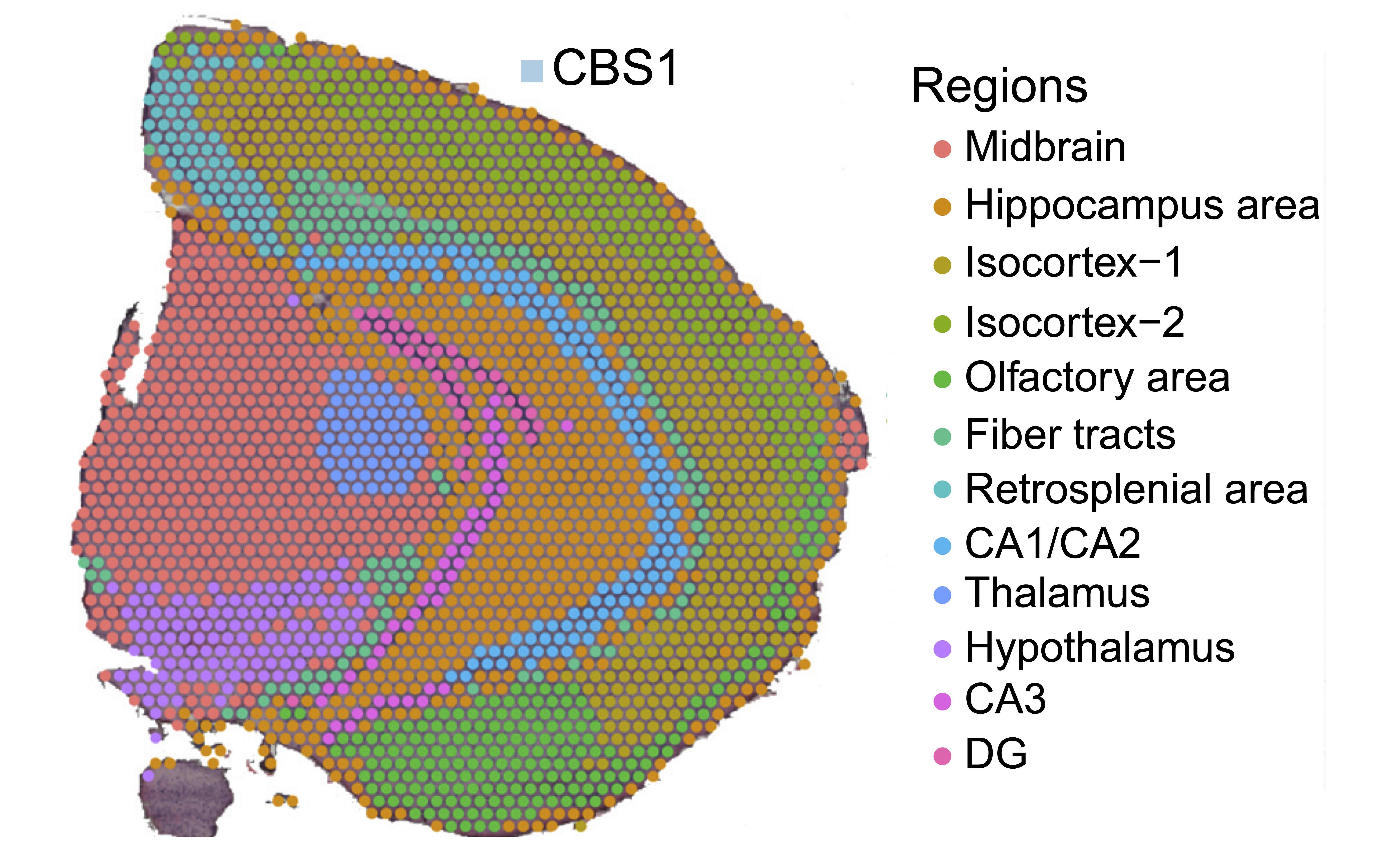
Analyzed spatial transcriptomics data from the SiT Mouse Brain dataset (CBS1_illu) by Lebrigand et al., 2023, which captures gene expression patterns with spatial context from mouse brain samples. The dataset comprises:
- 2,560 spatial spots representing distinct tissue locations
- 31,053 genes, filtered to 3,000 highly variable genes (HVGs)
- Spatial coordinates preserving tissue architecture
- 13 annotated cell types/regions including CA1/CA2, CA3, DG, Hippocampus, Hypothalamus, Isocortex, and others
Research Question: How do different self-supervised learning (SSL) approaches perform when combined with graph neural networks (GNNs) for learning spatial transcriptomics representations?
Graph Construction
As detailed in my previous work on GNNs for spatial transcriptomics, I constructed a k-nearest neighbor spatial graph (k=8) based on Euclidean distances between spot coordinates, resulting in 2,560 nodes and 40,960 edges.
Methods
GNN Architectures
Three GNN architectures were evaluated as encoder backbones:
- GraphSAGE (SAGEConv): Samples and aggregates features from neighbors using mean pooling
- Graph Attention Networks (GATConv): Learns attention weights to weigh neighbor importance (4 attention heads)
- Graph Convolutional Networks (GCNConv): Applies spectral graph convolutions for feature aggregation
Architecture specifications:
- 2 GNN layers
- Hidden dimension: 256
- Projection dimension: 64
- Batch normalization and dropout (0.1) between layers
Self-Supervised Learning Methods
Eight state-of-the-art SSL methods were compared across different families:
Contrastive Learning:
- SimCLR: Contrastive learning using NT-Xent loss (temperature=0.2)
- SwAV: Swapping assignments between views using optimal transport (512 prototypes)
Momentum-based Methods:
- BYOL: Bootstrap Your Own Latent without negative pairs (momentum=0.99)
- MoCo: Momentum contrast with a queue of negative samples (queue size=4096, momentum=0.99)
- SimSiam: Simple Siamese Networks with stop-gradient
Reconstruction-based:
- MAE: Masked Autoencoder reconstructing masked gene expressions (mask ratio=0.75)
Redundancy Reduction:
- Barlow Twins: Self-supervised learning via redundancy reduction (λ=0.005)
- VICReg: Variance-Invariance-Covariance Regularization (λ_inv=25, λ_var=25, λ_cov=1)
Data Augmentation: Gene dropout (10%) and Gaussian noise addition (scale=0.005)
Training: 20 epochs, batch size 256, AdamW optimizer (lr=1e-4, weight decay=1e-5)
Evaluation Metrics
Five complementary metrics were used to evaluate 24 method-backbone combinations:
- AMI/NMI (Adjusted/Normalized Mutual Information): Clustering agreement with ground truth annotations
- Silhouette Score: Internal cluster cohesion and separation
- Moran's I: Global spatial autocorrelation (higher = stronger spatial coherence)
- Geary's C: Alternative spatial autocorrelation measure (lower = stronger spatial coherence)
Important Note: These metrics provide a partial view of model performance. They don't capture robustness to batch effects, transferability to downstream tasks, biological interpretability, or performance on rare cell types.
Results
Clustering Visualizations by Backbone
The spatial clustering results reveal substantial qualitative differences across methods and backbones:
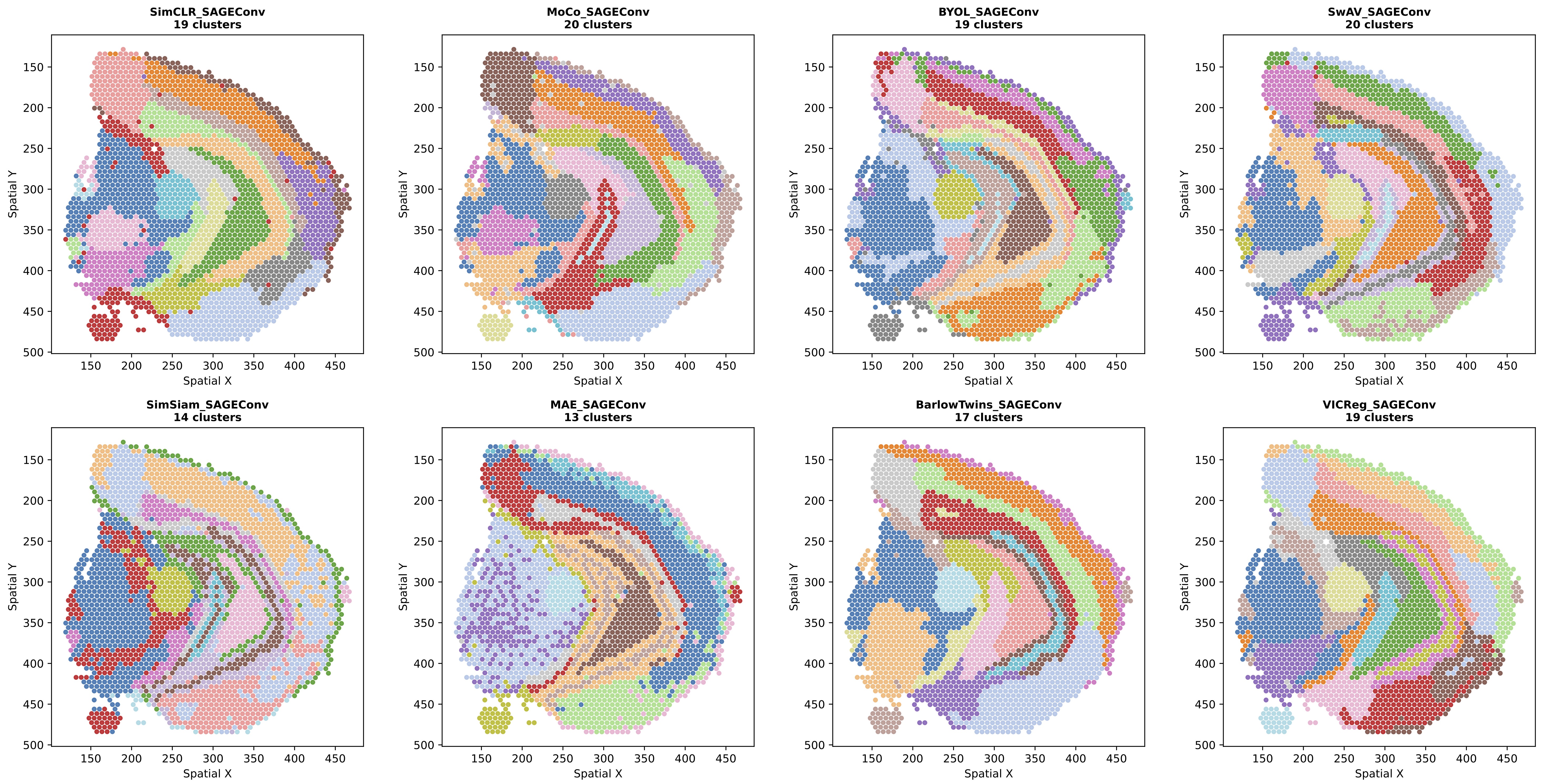 Figure 1: Leiden clustering results for all SSL methods using SAGEConv backbone. SAGEConv-based methods tend to produce more fragmented spatial patterns with sharper local transitions, potentially preserving fine-grained local heterogeneity.
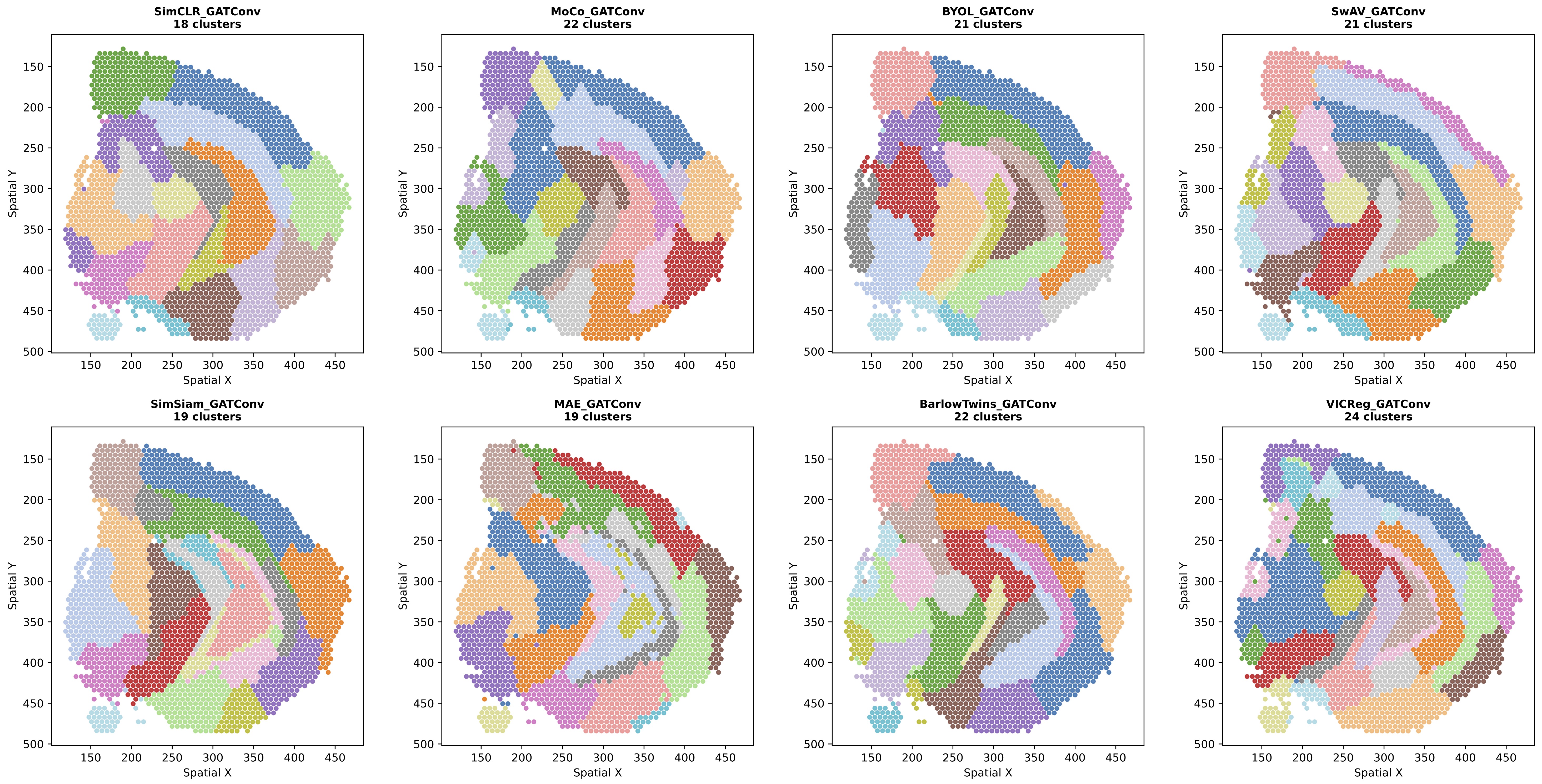 Figure 2: Leiden clustering results for all SSL methods using GATConv backbone. GATConv shows intermediate behavior with learned attention weights adding flexibility to adapt to local structure.
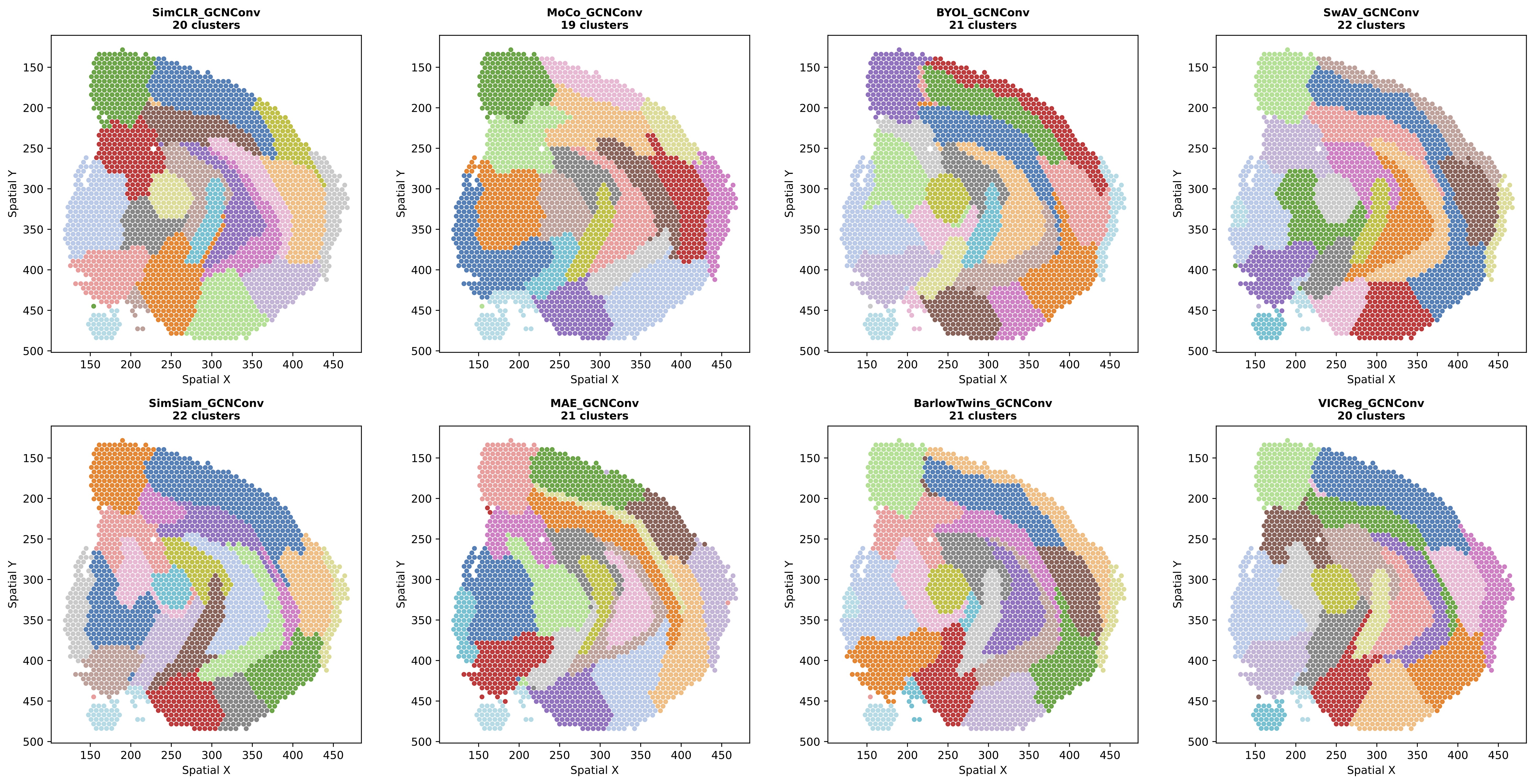 Figure 3: Leiden clustering results for all SSL methods using GCNConv backbone. GCNConv-based methods generally show more spatially contiguous clusters with smoother boundaries and stronger delineation along major anatomical boundaries.
Quantitative Performance Metrics
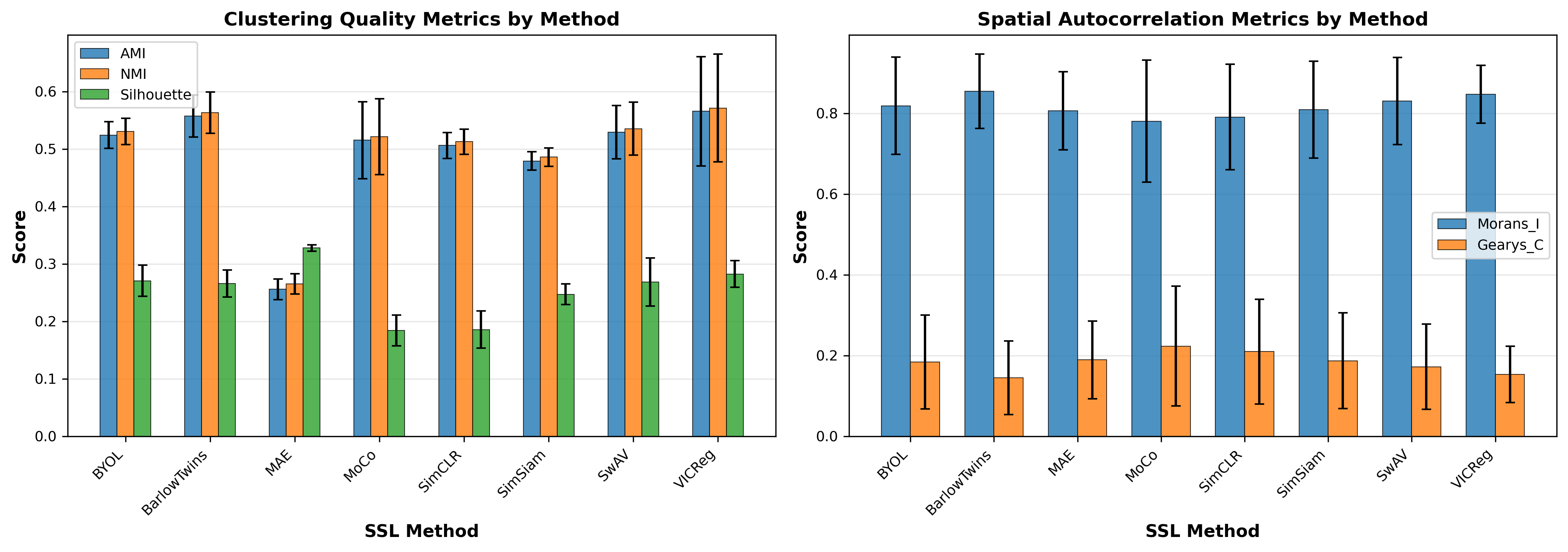 Figure 4: Average performance by SSL method across clustering and spatial metrics. Redundancy reduction methods (VICReg, Barlow Twins) show higher clustering agreement, while methods vary substantially in spatial autocorrelation.
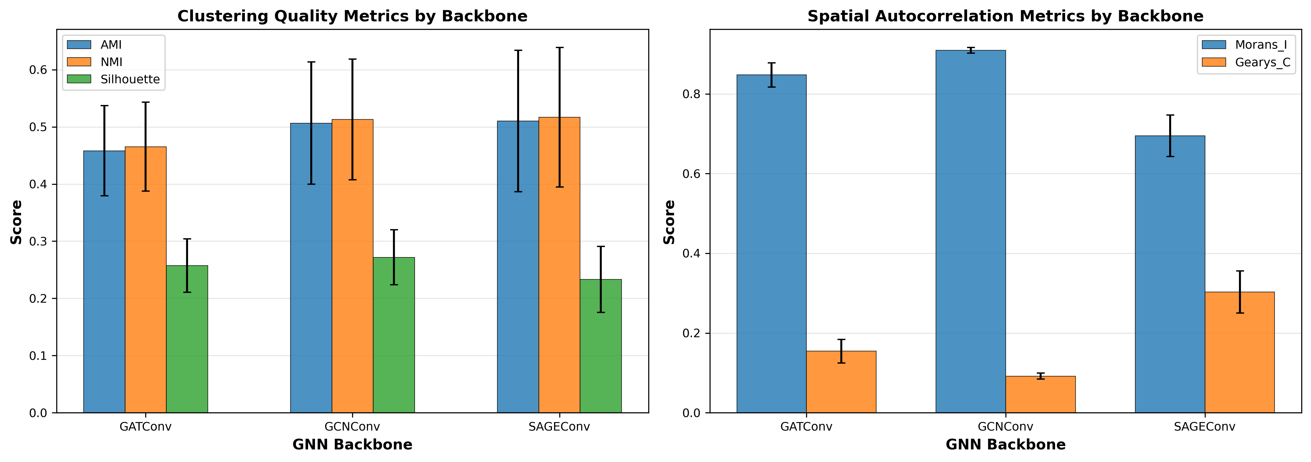 Figure 5: Average performance by GNN backbone. GCNConv shows very low variance in spatial metrics, suggesting strong spatial smoothing. SAGEConv exhibits highest variance across methods, indicating SSL objective matters more for this backbone.
Method Performance Summary
Average behavior across all three GNN backbones (mean ± std):
| Method | AMI | NMI | Silhouette | Moran's I | Geary's C |
|---|---|---|---|---|---|
| VICReg | 0.566±0.095 | 0.572±0.094 | 0.283±0.023 | 0.847±0.072 | 0.153±0.070 |
| Barlow Twins | 0.558±0.036 | 0.563±0.036 | 0.266±0.024 | 0.855±0.092 | 0.145±0.091 |
| SwAV | 0.529±0.047 | 0.536±0.046 | 0.269±0.042 | 0.830±0.108 | 0.172±0.106 |
| BYOL | 0.524±0.023 | 0.531±0.023 | 0.271±0.027 | 0.819±0.121 | 0.184±0.116 |
| MoCo | 0.515±0.067 | 0.522±0.066 | 0.184±0.027 | 0.781±0.151 | 0.224±0.148 |
| SimCLR | 0.506±0.022 | 0.513±0.022 | 0.186±0.033 | 0.791±0.130 | 0.210±0.129 |
| SimSiam | 0.479±0.016 | 0.486±0.016 | 0.247±0.018 | 0.809±0.120 | 0.187±0.119 |
| MAE | 0.256±0.018 | 0.265±0.018 | 0.328±0.006 | 0.806±0.097 | 0.189±0.096 |
Metric Relationships
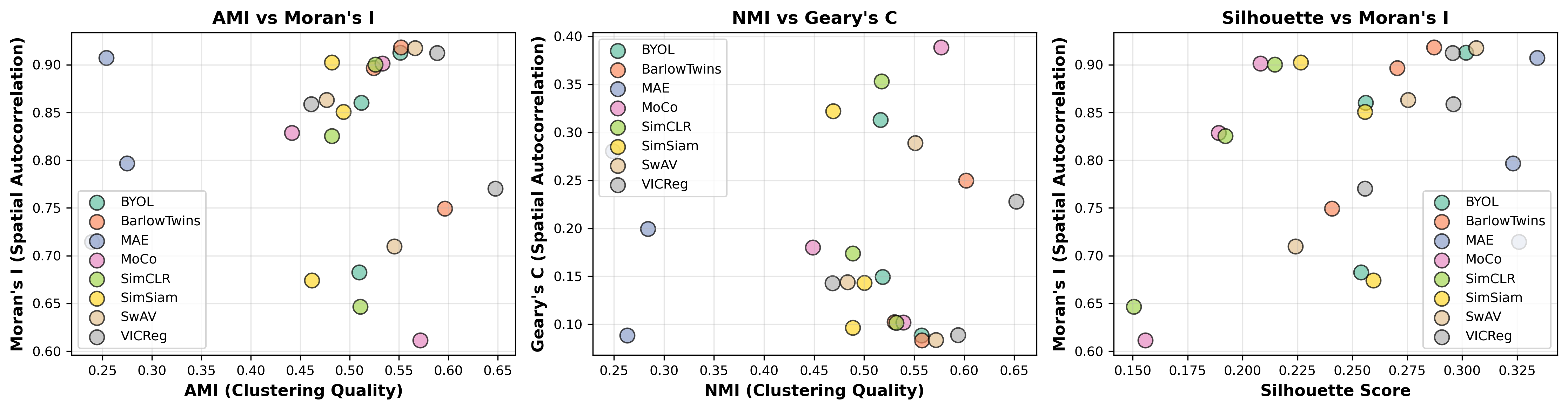 Figure 6: Relationships between clustering quality and spatial coherence metrics. AMI vs. Moran's I show positive correlation (ρ≈0.75), though this may reflect GCNConv's strong influence on both metrics.
Key Findings
Observed Patterns
BYOL with SAGEConv shows promise: This combination achieves balanced performance across metrics (AMI=0.510, NMI=0.516, Silhouette=0.254, Moran's I=0.683) without over-optimizing for any single one, suggesting potential for further investigation.
Redundancy reduction methods show consistency: VICReg and Barlow Twins exhibit higher AMI/NMI values and more consistent behavior across backbones (lower std), suggesting robust learning dynamics.
BYOL demonstrates remarkable consistency: With std=0.023 for AMI across different GNN architectures, BYOL's momentum-based approach appears robust to architectural choices.
MAE exhibits a paradox: Highest Silhouette scores (0.328) but lowest clustering agreement (AMI=0.256). This suggests it learns internally coherent representations that don't align with the provided annotations. It maybe suffering from the "noise"?
Strong method-backbone interactions: The same SSL method behaves very differently depending on GNN backbone, with variance up to 0.124 in AMI, indicating that architecture choice significantly influences representation learning.
GNN Backbone Trade-offs
GCNConv: Shows very low variance in spatial metrics (std=0.007 for Moran's I), suggesting spectral operations impose strong spatial smoothing regardless of SSL method. This high spatial coherence may be desirable or may indicate over-smoothing.
SAGEConv: Exhibits comparable AMI to GCNConv (0.510 vs. 0.507) but lower spatial autocorrelation (Moran's I=0.695). Highest variance across methods (std=0.124) indicates SSL objective matters more for this backbone, potentially preserving local heterogeneity (can also be observed from Figure 1~3).
GATConv: Shows intermediate values across all metrics with learned attention weights providing flexibility to adapt to local structure. As a side project, I experimented with adding regional attention mechanisms that provide the model with global spatial relationships, which significantly improved GAT's performance across all metrics.
Key Findings
Critical Limitations
This exploratory study has important limitations that constrain conclusions:
Evaluation Limitations:
- Metrics are proxies, not ground truth—AMI/NMI assume the 13 annotated regions are "correct," but annotations may be incomplete or subjective
- Single dataset from mouse brain may not generalize to other tissues or organisms
- Limited hyperparameter exploration (only 20 epochs, fixed augmentation parameters)
- No downstream task evaluation for actual biological utility
- Small dataset (2,560 spots) may not reveal scalability issues
Interpretation Challenges: High Moran's I could reflect beneficial spatial structure or excessive smoothing. High Silhouette doesn't guarantee biological relevance. Therefore, these metrics primarily identify differences in learned representations rather than definitively ranking method quality.
Potential Hybrid Approaches
Given different strengths of each method family, combining approaches may be promising:
SimCLR + Barlow Twins: Combine discriminative learning through contrastive loss with decorrelation to prevent feature redundancy. This may achieve both strong discrimination and feature diversity without collapse.
BYOL + VICReg: Add VICReg's variance/covariance terms to BYOL's predictor objective to provide explicit collapse prevention mechanism while maintaining momentum-based stability.
Spatial-aware SSL: Add explicit spatial regularization term to existing methods to test whether explicit spatial terms improve over implicit (GNN-based) spatial encoding.
Future Directions
Next Steps
Cross-tissue validation: The single-dataset limitation is this study's most critical weakness. Evaluation on diverse tissues (liver, heart, tumor microenvironments) and larger datasets (10,000+ spots) is essential to assess generalizability and scalability.
Biological validation: Beyond clustering metrics, I plan to evaluate differential gene expression, pathway enrichment, rare cell type recovery, and spatial trajectory inference quality to assess actual biological utility.
Hybrid method development: Systematic investigation of combined approaches (SimCLR+Barlow Twins, BYOL+VICReg) with careful hyperparameter tuning may leverage complementary strengths.
Downstream task evaluation: Test representations on actual biological questions including differential expression analysis, cell-cell communication, and trajectory inference.
Open Questions
- Why does BYOL-SAGEConv show such balanced behavior across metrics?
- Can we design metrics that better reflect biological utility rather than statistical properties?
- How do methods perform on rare cell types not well-represented in the dataset?
- What is the minimal dataset size needed for each method to perform effectively?
- Can we predict which method suits a given tissue type a priori?
- Can we treat gene expression patterns as samples instead of spots? Currently, each spot (with its gene expression vector) is treated as a sample. An alternative approach would be to treat each gene's expression pattern across all spots as a sample—essentially viewing each gene as an "image" where pixel intensities represent expression levels at different spatial locations. This gene-centric perspective might reveal different biological insights about co-expression patterns and spatial gene regulatory networks.
Conclusion
This systematic comparison of 8 self-supervised learning methods across 3 GNN architectures reveals substantial differences in how representations are learned for spatial transcriptomics data. While definitive conclusions about method superiority require more comprehensive evaluation, several patterns emerged:
- Substantial method-backbone interactions with the same SSL method behaving very differently depending on GNN backbone
- BYOL-SAGEConv shows balanced performance across diverse metrics without over-optimizing for any single one
- Redundancy reduction methods (VICReg, Barlow Twins) demonstrate consistency across architectures
- Evaluation challenges highlight the difficulty of assessing representation quality through clustering and spatial metrics alone
Future work will focus on cross-tissue validation, biological validation through downstream tasks, and development of hybrid approaches that combine complementary strengths of different SSL families.
Acknowledgments
This analysis leveraged:
- SiT Mouse Brain dataset for spatial transcriptomics data
- PyTorch Geometric for GNN implementations
- Scanpy for preprocessing and visualization
- Scikit-learn for evaluation metrics
References
SSL Methods:
- Chen et al. (2020) - SimCLR: A Simple Framework for Contrastive Learning
- He et al. (2020) - MoCo: Momentum Contrast for Unsupervised Visual Representation Learning
- Grill et al. (2020) - BYOL: Bootstrap Your Own Latent
- Caron et al. (2020) - SwAV: Unsupervised Learning of Visual Features by Contrasting Cluster Assignments
- Chen & He (2021) - SimSiam: Exploring Simple Siamese Representation Learning
- He et al. (2022) - MAE: Masked Autoencoders Are Scalable Vision Learners
- Zbontar et al. (2021) - Barlow Twins: Self-Supervised Learning via Redundancy Reduction
- Bardes et al. (2022) - VICReg: Variance-Invariance-Covariance Regularization
GNN Architectures:
- Hamilton et al. (2017) - GraphSAGE: Inductive Representation Learning on Large Graphs
- Veličković et al. (2018) - GAT: Graph Attention Networks
- Kipf & Welling (2017) - GCN: Semi-Supervised Classification with Graph Convolutional Networks
Spatial Transcriptomics:
- Lebrigand et al. (2023) - The spatial landscape of gene expression isoforms in tissue sections