What a Frozen Pathology Encoder Already Knows
A whole-slide benchmark on 2,099 public TCGA slides showed that a frozen foundation encoder plus mean pooling and a linear head recovers receptor status and HRD from H&E. A more complex learned-attention aggregator did not beat that simple baseline: it piled nearly all of its weight onto ~10% of tiles and gained no accuracy for it.
Disclosure note. All data are public TCGA-BRCA and TCGA-OV whole-slide images and public derived label tables; no internal cohort, patient-level record, or infrastructure detail is included. Reported values are cross-validated aggregates. Predictions are research outputs, not clinical assays.
What a Frozen Pathology Encoder Already Knows
A whole-slide image is a gigapixel scan of one glass slide. The molecular label you want to predict — receptor status, a genomic-instability score — belongs to the patient, not to any 224-pixel patch of it. Nobody annotates tiles at cohort scale, so the supervision is weak by construction.
That makes the interesting question narrower than "can a network predict molecular labels from H&E." It is:
How much of that signal is already present in a general-purpose pathology representation, before we train anything — and does a learned aggregator earn its complexity on top of it?
I built the benchmark to answer that with controls rather than a single headline number. The result: a frozen encoder plus mean pooling plus a linear head recovers ER, TNBC and HRD at levels that survive leave-institution-out validation. A gated-attention aggregator, after I retrained it to recover the per-tile weights the first run discarded, does not beat that mean — and the reason is visible in its attention distribution.
Table of contents
- Problem framing
- Pipeline
- Formulas
- Endpoint tiering
- What the frozen representation encodes
- Discrimination across endpoints
- Regression and error structure
- Does attention earn its complexity
- Per-tile evidence
- Generalization to unseen institutions
- The tumor-purity confound
- What each aggregator actually learns
- Limitations
- Take-home
- References
Problem framing
This is a multiple instance learning (MIL) problem. A patient is a bag; each tile is an instance; only the bag carries a label. Two design decisions follow, and both turned out to matter more than model choice:
- Bag at the patient level, not the slide level. A third of patients (484 of 1,485) have more than one slide — multiple tissue samples, or multiple sections of the same block. Bagging per slide would manufacture duplicate labels and let one patient's slides land on both sides of a split.
- Freeze the encoder. Then every result is a statement about the representation, not about a network tuned to these endpoints — and the aggregator comparison is clean, because both arms consume identical features.
Pipeline
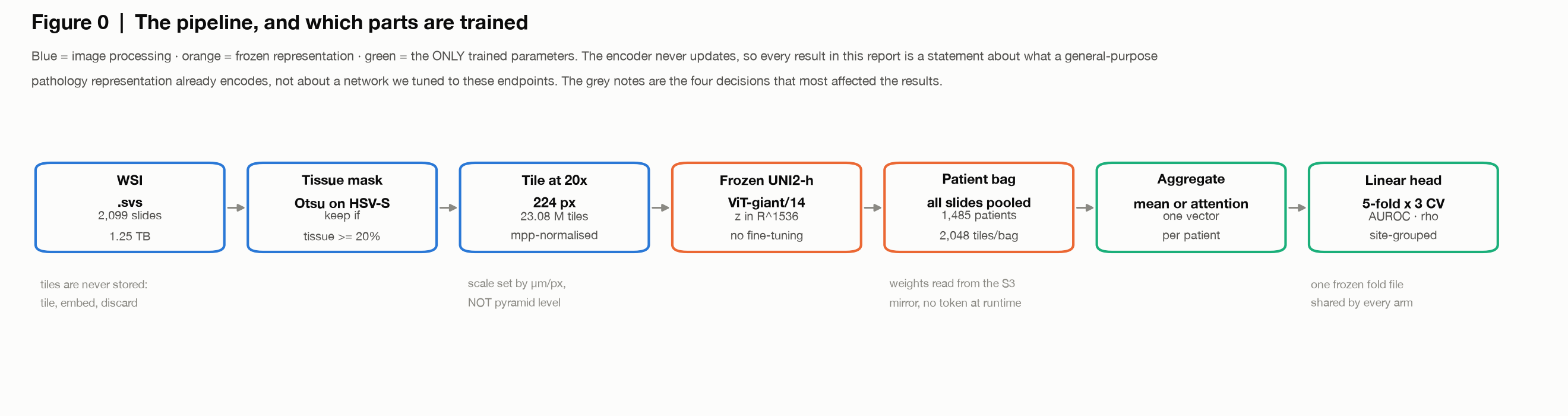
2,099 slides (1,130 TCGA-BRCA FFPE-diagnostic, 969 TCGA-OV frozen sections) → 23.08 M tiles → 66 GB of embeddings. Tiles are never persisted: tile, embed, discard. That is why a 1.25 TB slide corpus reduces to 66 GB of features instead of multiple TB of JPEGs.
Three implementation details carried disproportionate weight:
- Scale normalization by microns-per-pixel, not pyramid level. TCGA mixes 20× and 40× scans, so "level 0" is not a consistent magnification. Getting this wrong silently feeds the encoder tissue at two different physical scales.
- Architecture read from each model's own config, never hardcoded. Doing this caught four real loading bugs, including a wrong ViT variant and mishandled register tokens that would have averaged non-patch tokens into the pooled feature.
- Row-contiguous HDF5 chunking. Auto-chunking split the 1,536-d feature axis into 32 pieces, so reading one tile meant 32 chunk reads. Measured effect: 40 IOPS and 93% disk utilization at 87% CPU idle. Fixing the chunk shape took the training phase from a projected ~30 hours to ~55 minutes.
Formulas
Each stage as actually applied, in order:
(1)  tissue mask        M(x,y) = 1[ S(x,y) > tau_Otsu ]          S = HSV saturation
(2)  tile accept        keep tile iff  mean(M) >= 0.20  AND  std(x) >= 8
(3)  scale normalize    s = mpp_target / mpp_0,   p_read = round(T * s)
(4)  frozen encoder     z_i = f(x_i) in R^1536,   grad(f) == 0
(5)  patient bag        Bag(p) = { z_i : z_i in slide s,  for all slides s of p }
(6)  mean pooling       z_bar = (1/N) * sum_i z_i
(7)  linear head        y_hat = sigmoid( w . z_bar + b )
(8)  gated attention    a_i = softmax_i( w_a^T [ tanh(V h_i) * sigmoid(U h_i) ] )
                        z_tilde = sum_i a_i h_i
(9)  attribution        w . z_bar + b == (1/N) * sum_i ( w . z_i + b )
(10) evaluation         5-fold x 3 repeats, patient-level, stratified;
                        site-grouped variant = StratifiedGroupKFold on source site
Line (9) is the one to notice. It is an algebraic identity, not an approximation:
because the head is linear and the aggregator is a mean, a patient's score is the mean
of per-tile contributions c_i = w . z_i + b. That makes mean pooling exactly
decomposable, which is what makes the evidence maps below a decomposition rather than a
saliency heuristic.
Line (8) softmaxes over instances, not features — the standard gated-attention MIL formulation.
Endpoint tiering
Endpoints were tiered by whether they are orthogonal to bulk RNA, because that determines what a good score can be used to argue:
| Tier | Endpoint | Measured by | n |
|---|---|---|---|
| A · protein | ER, TNBC | immunohistochemistry | 1,009 / 915 |
| A · DNA | HRD binary, HRD score | genomic scarring (LOH/TAI/LST) | 927 |
| A · DNA | OV HRD | same, ovarian | 173 |
| B · circular | PAM50 | called from bulk mRNA | 950 |
PAM50 is reported for completeness only. It is derived from bulk expression, so it cannot serve as independent evidence for any RNA-related claim — a distinction that is easy to lose when every endpoint is just another column in a results table.
What the frozen representation encodes
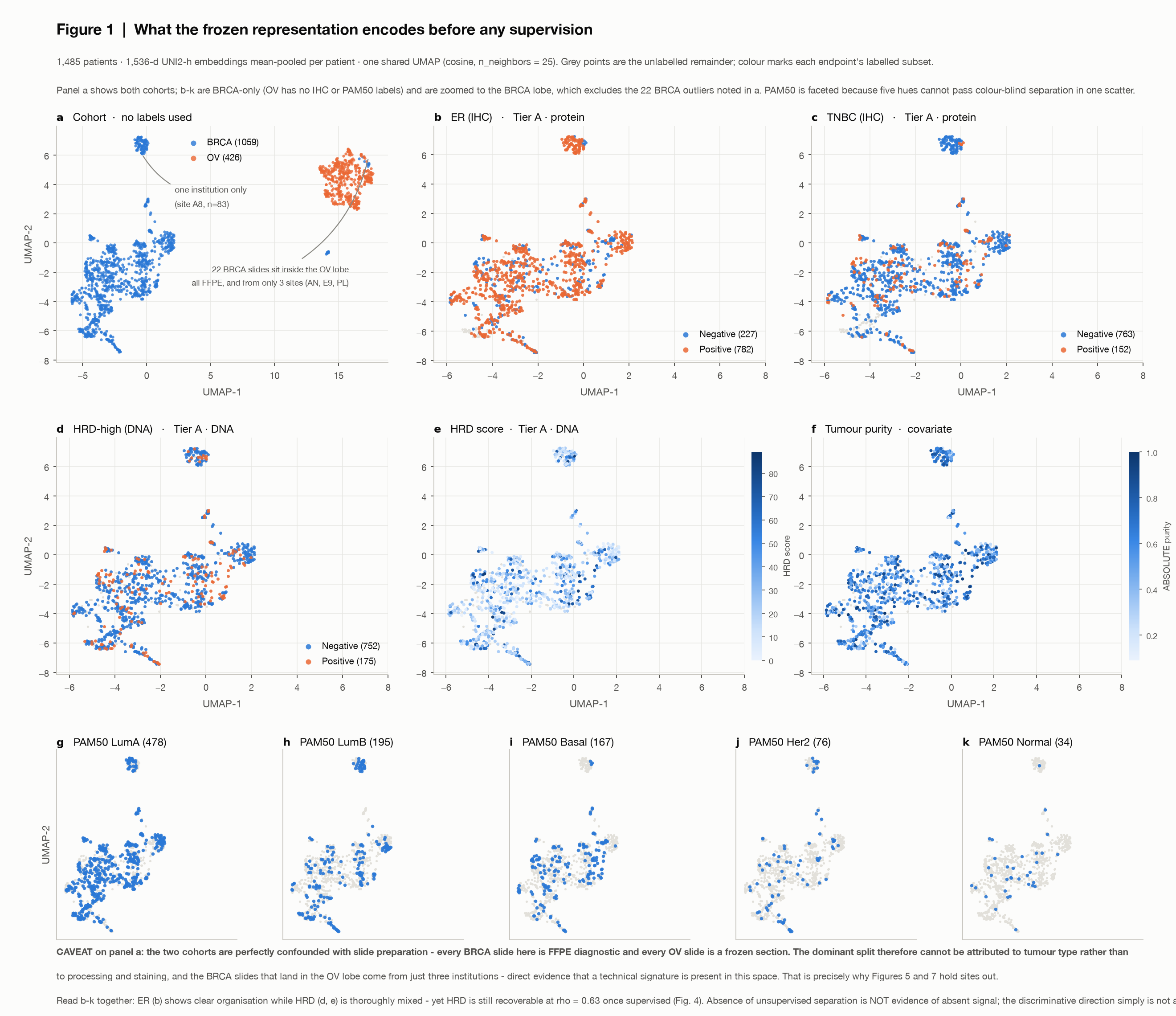
One shared UMAP of mean-pooled patient embeddings, colored by each endpoint in turn. Two things are worth reading carefully.
The cohort split is confounded with slide preparation. Every BRCA slide here is FFPE and every OV slide is a frozen section, so the dominant axis cannot be attributed to tumor type rather than to processing and staining. Supporting evidence sits in the same panel: 22 BRCA slides land inside the OV lobe, all FFPE, drawn from only three institutions. A technical signature demonstrably exists in this space.
Absence of unsupervised separation is not absence of signal. HRD is thoroughly mixed in the unsupervised view, yet it is recoverable at ρ ≈ 0.63 once supervised. The discriminative direction simply is not among the top variance directions — which is the whole reason a supervised probe is informative and a UMAP alone is not.
Discrimination across endpoints
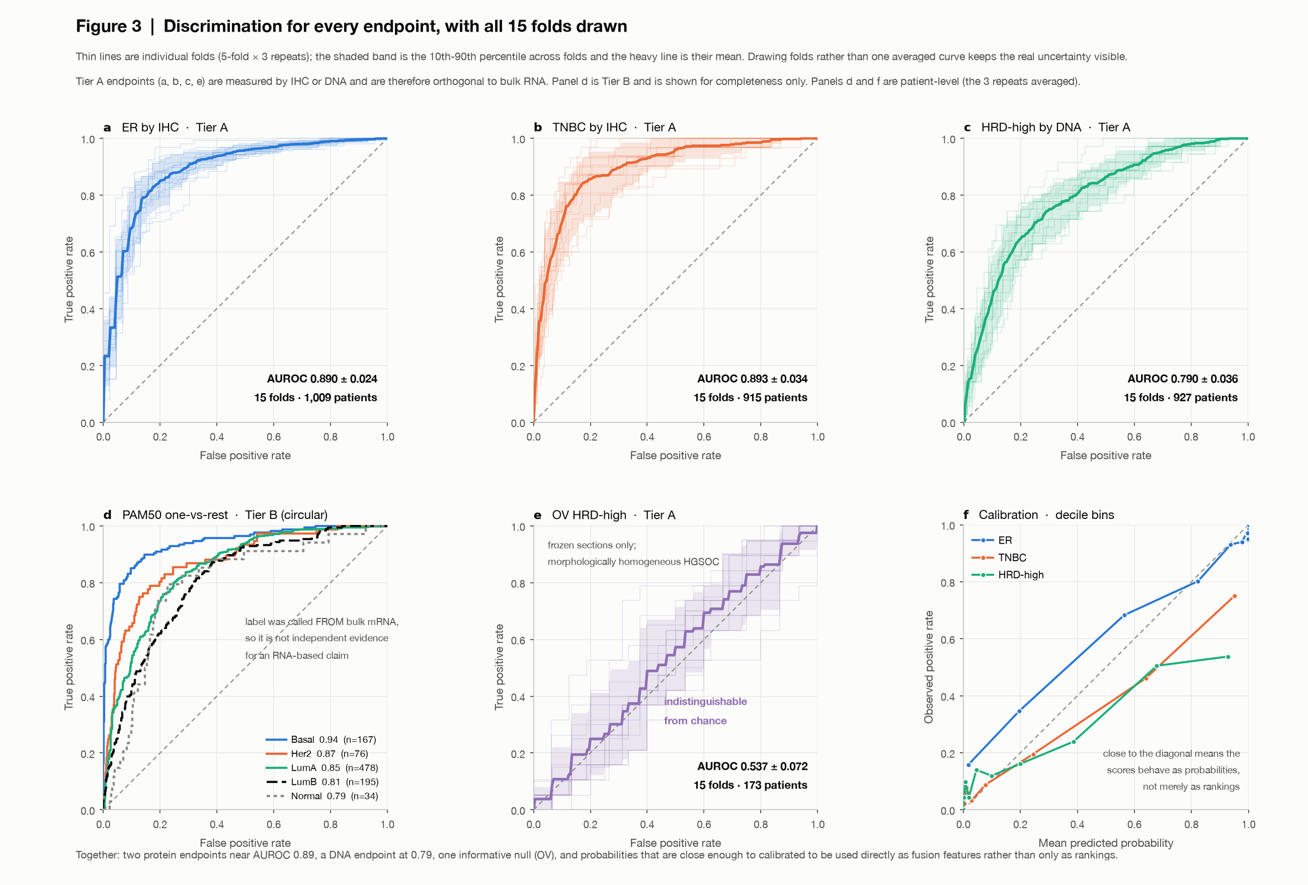
Mean pooling with a linear head, all 15 folds drawn rather than one averaged curve:
| Endpoint | Tier | Patient-random | Site-grouped |
|---|---|---|---|
| ER by IHC | A · protein | 0.890 ± 0.024 | 0.875 ± 0.050 |
| TNBC by IHC | A · protein | 0.893 ± 0.034 | 0.865 ± 0.060 |
| HRD binary | A · DNA | 0.790 ± 0.036 | 0.806 ± 0.059 |
| HRD score (ρ) | A · DNA | 0.622 ± 0.033 | 0.610 ± 0.104 |
| PAM50 (OvR) | B · circular | 0.809 ± 0.027 | 0.789 ± 0.046 |
| OV HRD | A · DNA | 0.537 ± 0.072 | 0.514 ± 0.120 |
AUROC unless noted; ± SD over 15 folds.
Under site-grouped cross-validation — no institution in both train and test — every drop is ≤ 0.03 and HRD-high slightly improves. This is the control that matters most for TCGA whole-slide work, which is routinely criticized for learning site and stain signatures. The signature exists (previous figure); the label-relevant directions do not depend on it.
The calibration panel is the practically useful one: the probabilities track the diagonal closely enough to be consumed as probabilities in a downstream model, not merely as rankings.
OV is an informative null. Chance in two independent formulations, with structural causes: frozen sections only, n = 173, and high-grade serous ovarian carcinoma is morphologically homogeneous. Reported as a negative result rather than omitted.
Regression and error structure
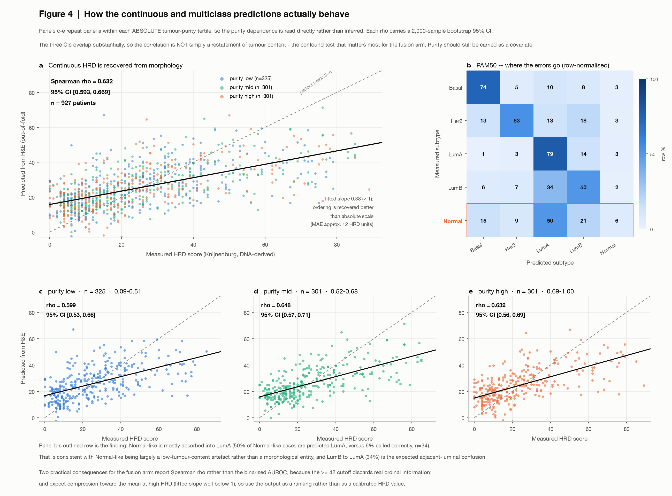
Two findings about how the predictions fail, which summary metrics hide.
Continuous HRD beats its binarized form (ρ 0.622 vs AUROC 0.790): the ≥ 42 cutoff discards real ordinal information. The fitted slope is well below 1, so the output recovers ordering far better than absolute scale — consume it as a ranking, not as a calibrated HRD value.
Normal-like PAM50 is largely a low-tumor-content artifact. 50% of Normal-like cases are predicted LumA versus only 6% called correctly (n = 34). Reporting PAM50 with and without Normal-like is therefore substantive, not cosmetic. Balanced accuracy across five classes is 0.523 — worth stating alongside the more flattering one-vs-rest AUROC of 0.809.
Does attention earn its complexity
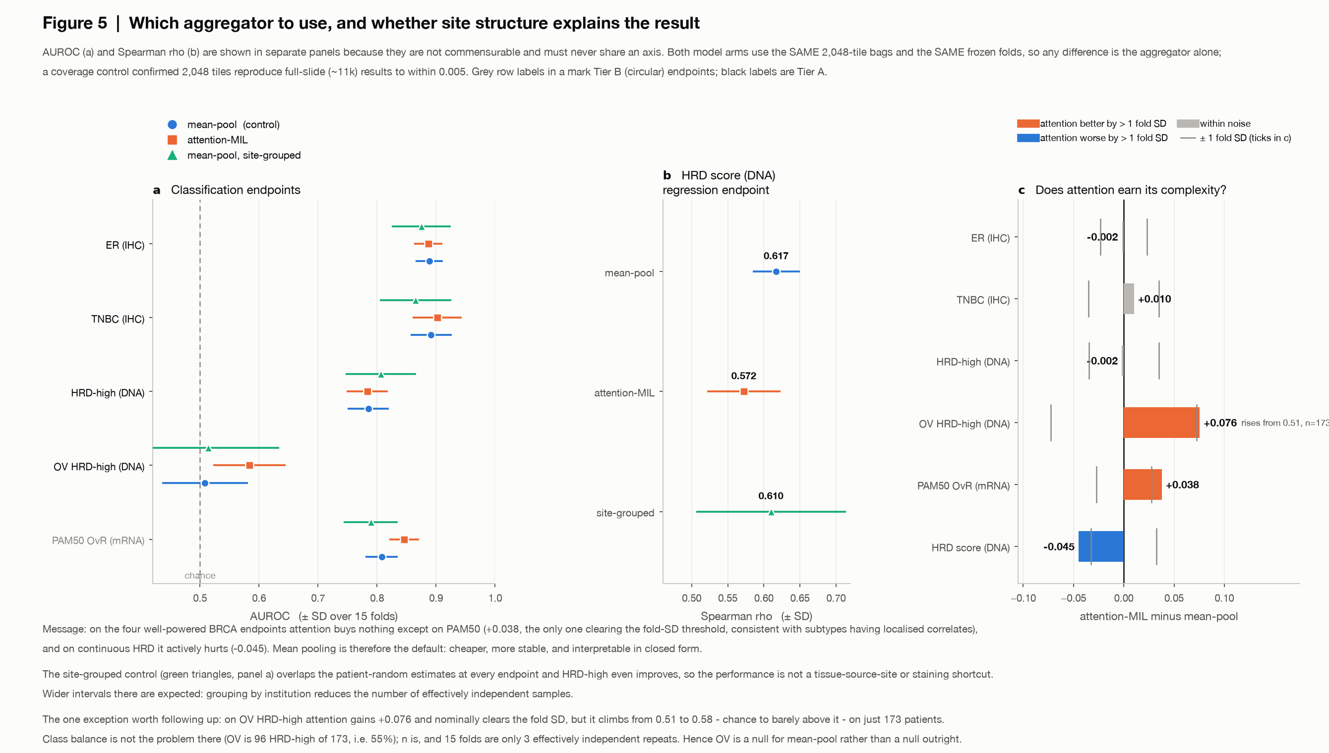
Both arms consume the same 2,048-tile bags and the same frozen folds, so any difference is the aggregator alone. A coverage control confirmed 2,048 tiles reproduce full-slide (~11k tiles) results to within 0.005 on all five BRCA endpoints — but by 0.029 on OV, another reminder that the small cohort is unstable rather than merely weak.
Judged against ±1 fold SD, on the four well-powered BRCA endpoints attention buys nothing except on PAM50 (+0.038), and on continuous HRD it actively hurts (−0.045).
The honest exception, stated as such: OV HRD gains +0.076, nominally clearing the fold SD — but it climbs from 0.51 to 0.58, chance to barely above it, on 173 patients where 15 folds are only 3 effectively independent repeats. Class balance is not the issue (OV is 96 HRD-high of 173). That is a re-check, not a result.
Mean pooling is the default: cheaper, more stable, and exactly decomposable.
Per-tile evidence
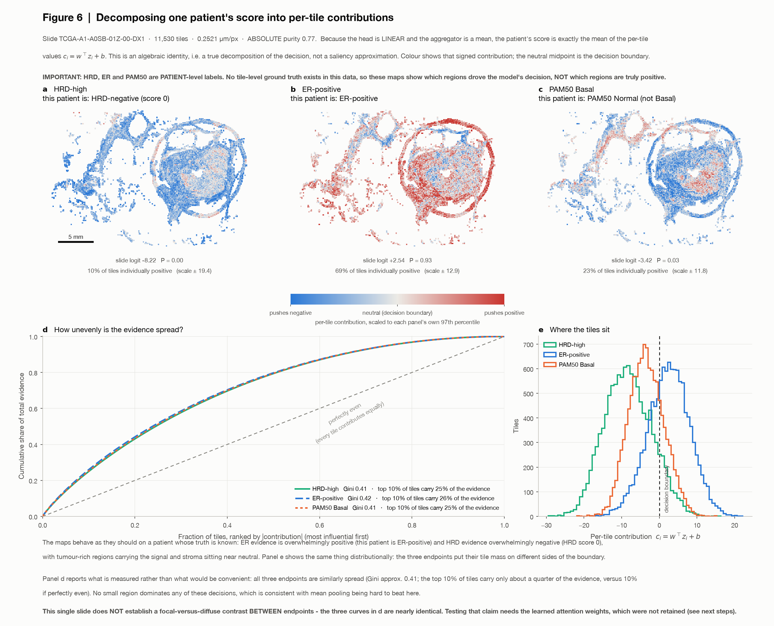
Using identity (9), one patient's score decomposes exactly into per-tile contributions. Color is the signed contribution; the neutral midpoint is the decision boundary.
What these maps are not: HRD, ER and PAM50 are patient-level labels, and no tile-level ground truth exists anywhere in this data — that is precisely why this is a MIL problem. The maps show which regions drove the model's decision, not which regions are truly positive. They are hypothesis-generating for pathologist review, not validated tile calls.
They do pass a sanity check on a patient whose truth is known: ER evidence is overwhelmingly positive (the patient is ER-positive), HRD evidence overwhelmingly negative (HRD score 0), with tumor-rich regions carrying the signal and stroma near neutral.
The concentration panel reports what was measured rather than what would have been convenient: all three endpoints are similarly diffuse (Gini ≈ 0.41; the top 10% of tiles carry only about a quarter of the evidence, versus 10% if perfectly even). No small region dominates — consistent with mean pooling being hard to beat. This single slide does not establish a focal-versus-diffuse contrast between endpoints; that needed the attention weights, below.
Generalization to unseen institutions
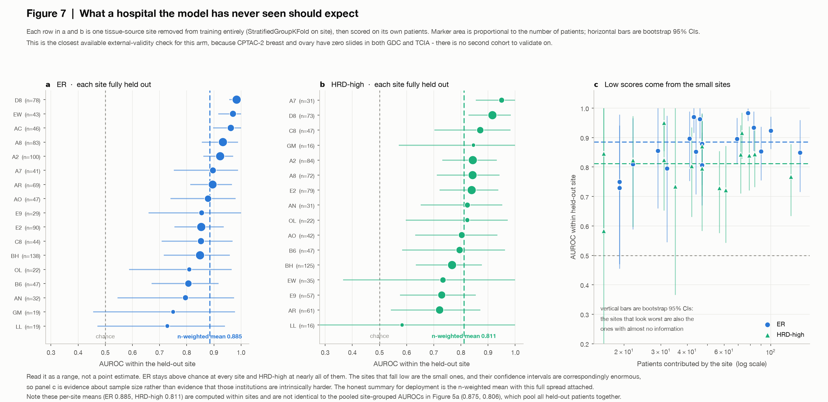
Each row is one tissue-source site removed from training entirely, then scored on its own patients. This is the ceiling on external validity for this cohort pair: CPTAC-2 breast and ovary have zero slides in both GDC and TCIA, so no second cohort exists to validate on.
Read as a range, not a point estimate. Point estimates stay above chance at every evaluable site — ER across 17 sites (n-weighted mean 0.885, minimum 0.729) and HRD-high across 16 (0.811, minimum 0.583) — though the bootstrap intervals of the smallest sites do cross 0.5. The sites that look worst are the small ones, and their intervals are enormous: that is evidence about sample size, not about those institutions being harder. The honest deployment summary is the n-weighted mean with this spread attached.
The tumor-purity confound
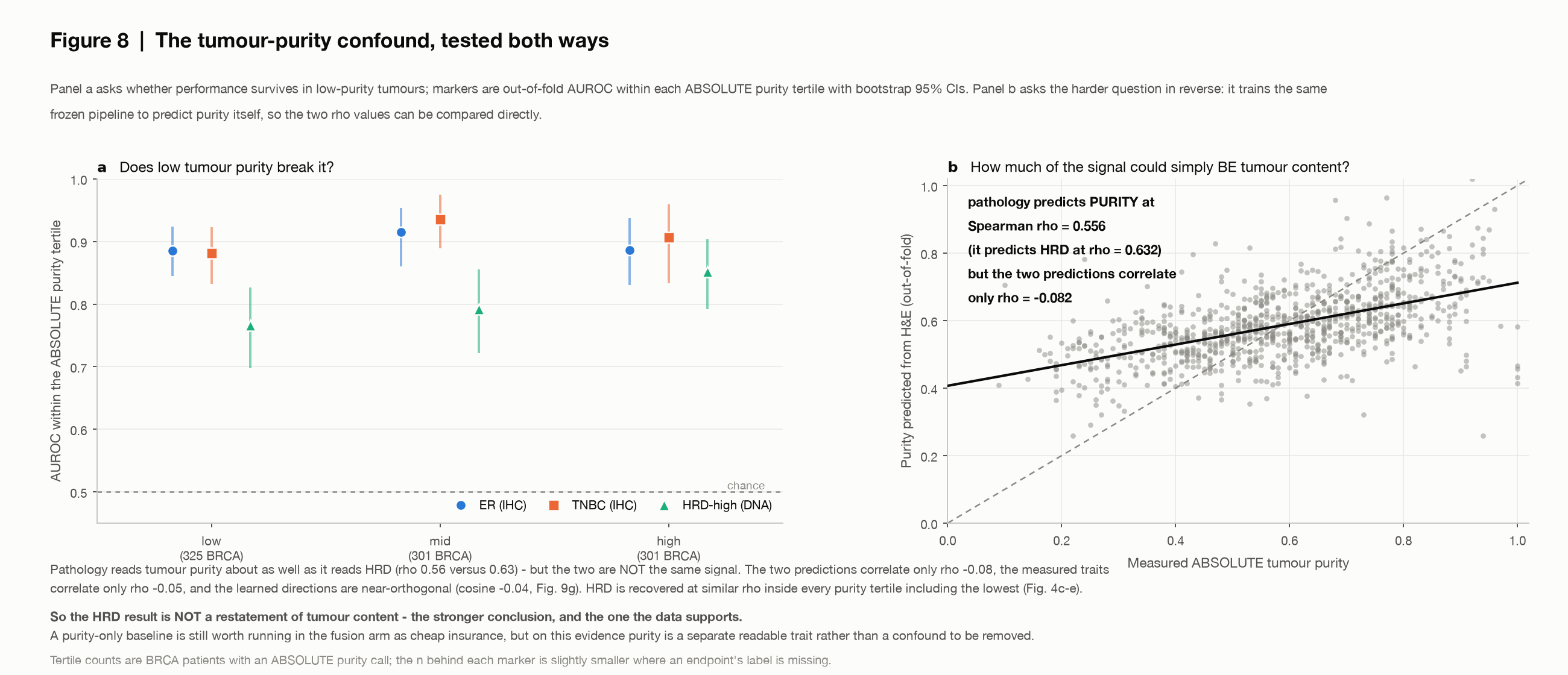
The obvious objection to any H&E-based molecular prediction is that the model is reading tumor content. I tested it in both directions.
Stratified: HRD-high runs 0.766 → 0.792 → 0.851 across purity tertiles — a real but modest gradient, still far above chance in the lowest tertile. ER and TNBC are flat. Continuous HRD is essentially flat too (ρ 0.599 / 0.648 / 0.632, overlapping bootstrap intervals).
Reversed: train the same frozen pipeline to predict purity itself. Pathology reads purity at ρ 0.556, about as well as it reads HRD at ρ 0.632.
Read alone, that looks damning. The next figure showed it is not.
What each aggregator actually learns
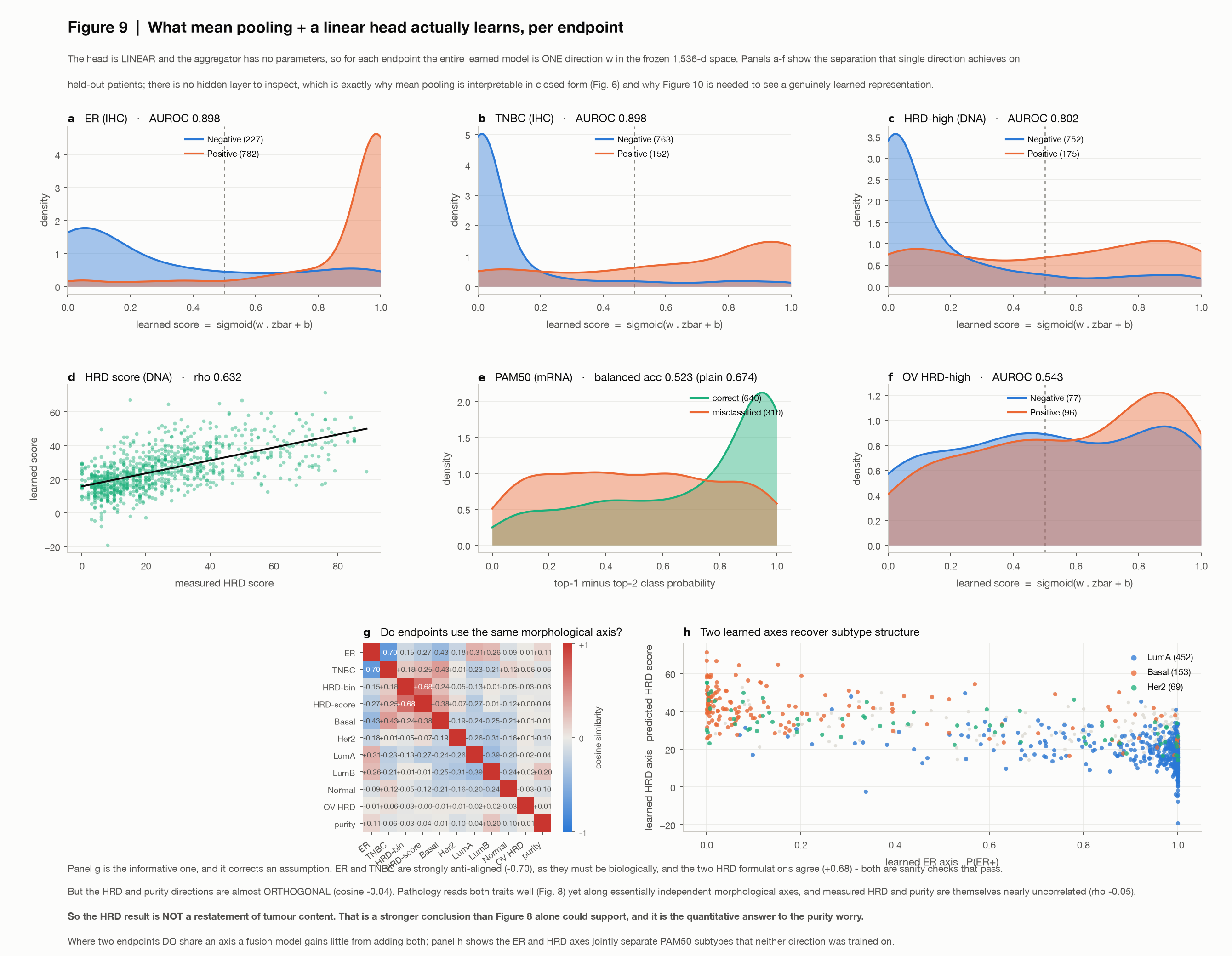
Because the head is linear and mean pooling has no parameters, the entire learned model for an endpoint is one direction w in the frozen space. That makes the models directly comparable to each other — just take cosine similarities.
Two sanity checks pass: ER and TNBC are strongly anti-aligned (−0.70), as biology requires, and the two HRD formulations agree (+0.68).
Then the correction. The HRD and purity directions are near-orthogonal (cosine −0.04). Pathology reads both traits well, but along essentially independent morphological axes: the two predictions correlate only ρ −0.08, and the measured traits themselves only −0.05. So the HRD result is not a restatement of tumor content. That is a stronger conclusion than the stratified analysis alone could support, and it replaced my earlier reading that the two signals were entangled.
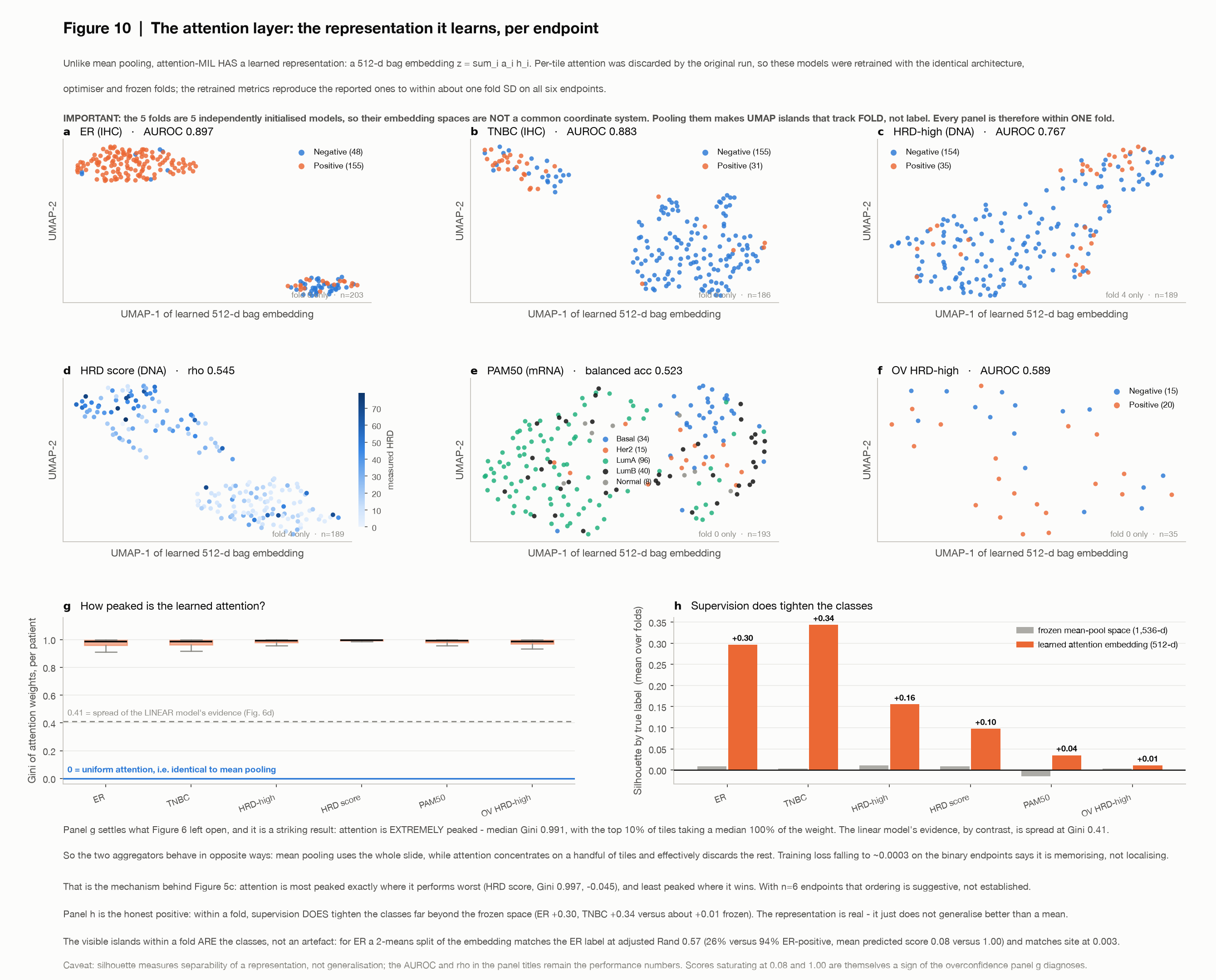
Attention-MIL, unlike mean pooling, has a learned representation: a 512-d bag embedding
z_tilde. The original run discarded the per-tile weights, so I retrained with identical
architecture, optimizer and folds; the retrained metrics reproduce the reported ones to
within about one fold SD on all six endpoints.
A correctness trap worth recording. The 5 folds are 5 independently initialized models, so their embedding spaces are not a common coordinate system. Pooling all out-of-fold embeddings into one UMAP produces tidy islands that look like biology but track fold (adjusted Rand 0.20–0.56 versus fold, ≈ 0.00 versus label). Every panel is therefore computed within a single fold. My first version of this figure had that bug.
Within a fold, the islands that remain are the classes: for ER, a 2-means split of the embedding matches the ER label at adjusted Rand 0.57 and matches site at 0.003.
The result that explains the aggregator comparison: attention is extremely peaked — median Gini 0.991, with the top 10% of tiles receiving a median ~100% of the weight. The linear model's evidence, by contrast, is spread at Gini 0.41. The two aggregators read a slide in opposite ways: mean pooling uses all of it, attention collapses onto a handful of tiles and discards the rest. Training loss falling to ~0.0003 on the binary endpoints says it is memorizing, not localizing. Attention is most peaked exactly where it performs worst (HRD score, Gini 0.997, −0.045); with six endpoints that ordering is suggestive, not established.
The honest positive is the last panel: within a fold, supervision does tighten the classes far beyond the frozen space (ER +0.30, TNBC +0.34 silhouette, versus ≈ +0.01 frozen). The learned representation is real. It simply does not generalize better than a mean.
Limitations
- Two cohorts from one consortium; no external pathology cohort exists for BRCA/OV, so leave-institution-out is the ceiling on external validity.
- Cohort and slide preparation are perfectly confounded (BRCA all FFPE, OV all frozen), so cross-cohort comparisons are not clean.
- OV is frozen-section only with n = 173; its null result is specific to that material and sample size.
- Tile-level maps are decompositions of model decisions, not validated tile-level calls — no tile-level ground truth exists.
- PAM50 is bulk-mRNA-derived and cannot support RNA-orthogonality claims.
- The attention retraining covers one repeat (5 folds) rather than all three.
- Purity and HRD are separable in this cohort's morphology; that should be re-tested before it is assumed elsewhere.
- One frozen encoder was evaluated end-to-end; encoder choice is uncontrolled.
Take-home
- A frozen pathology encoder plus mean pooling plus a linear head reaches AUROC 0.890 (ER), 0.893 (TNBC) and 0.790 (HRD-high) on labels measured by IHC and DNA — no fine-tuning anywhere in the stack.
- Those results survive leave-institution-out validation (every drop ≤ 0.03), even though a site signature is visibly present in the same embedding space.
- Continuous beats binarized for HRD (ρ 0.622 vs AUROC 0.790); thresholding at ≥ 42 discards real ordinal information.
- Learned attention did not earn its complexity. Recovering its discarded weights showed why: it concentrates ~100% of the weight on 10% of tiles (Gini 0.991) while the linear model's evidence is diffuse (0.41), and it memorizes rather than localizes.
- The tumor-purity objection was testable and answered: pathology predicts purity (ρ 0.556) along an axis nearly orthogonal to HRD (cosine −0.04), so the HRD signal is not a purity restatement.
- Two negatives worth publishing: OV HRD is at chance, and pooling per-fold embeddings into one UMAP manufactures fold-driven structure that is easy to mistake for biology.
References
- Chen, R. J. et al. Towards a general-purpose foundation model for computational pathology. Nature Medicine (2024).
- Ilse, M., Tomczak, J. M. & Welling, M. Attention-based deep multiple instance learning. ICML (2018).
- Lu, M. Y. et al. Data-efficient and weakly supervised computational pathology on whole-slide images. Nature Biomedical Engineering (2021).
- Knijnenburg, T. A. et al. Genomic and molecular landscape of DNA damage repair deficiency across The Cancer Genome Atlas. Cell Reports (2018).
- Aran, D., Sirota, M. & Butte, A. J. Systematic pan-cancer analysis of tumour purity. Nature Communications (2015).
- Parker, J. S. et al. Supervised risk predictor of breast cancer based on intrinsic subtypes. Journal of Clinical Oncology (2009).
- Howard, F. M. et al. The impact of site-specific digital histology signatures on deep learning model accuracy and bias. Nature Communications (2021).